Homework - Week 01

Q1

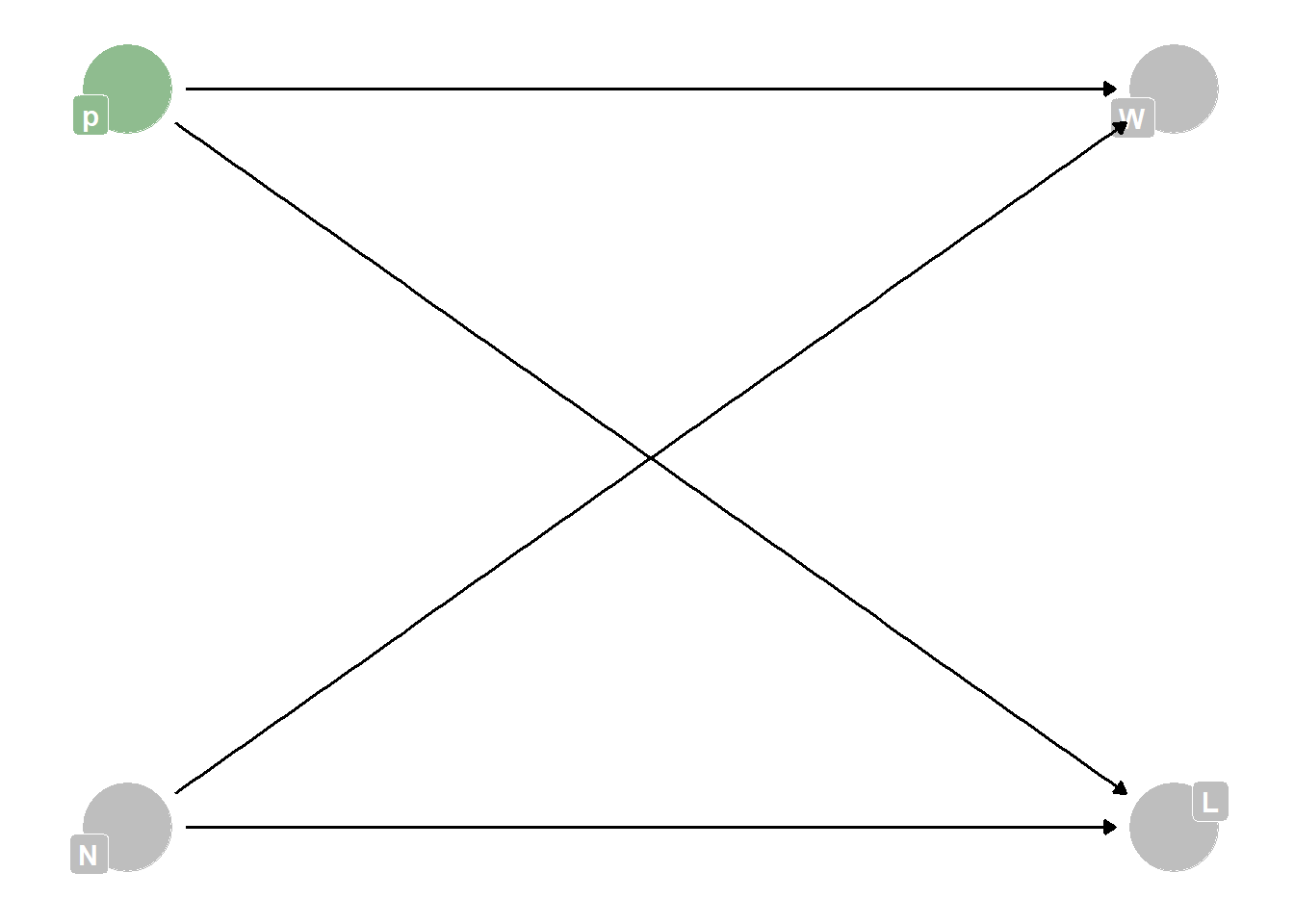
Suppose the globe tossing data had turned out to be 3 water and 11 land. Construct the posterior distribution.

DAG:

Posterior:

# create the sample manually
N_W <- 3
N_L <- 11
sample <- c(rep("W", N_W), rep("L", N_L))

# use compute_posterior with the sample function to compute the posterior 
compute_posterior <- function(the_sample, poss = seq(0, 1, length.out = 1000)){
  W <- sum(the_sample=="W")
  L <- sum(the_sample=="L")
  ways <- sapply(poss, function(q) (q*4)^W * ((1-q)*4)^L)
  post <- ways/sum(ways)
  #bars <- sapply(post, function(q) make_bar(q))
  data.frame(poss, ways, post = round(post, 3))
}

post <- compute_posterior(sample)

ggplot(post) + 
  geom_smooth(aes(x = poss, y = post), se = F) + 
  labs(y = "Posterior Probability", x = "p") + 
  theme_classic()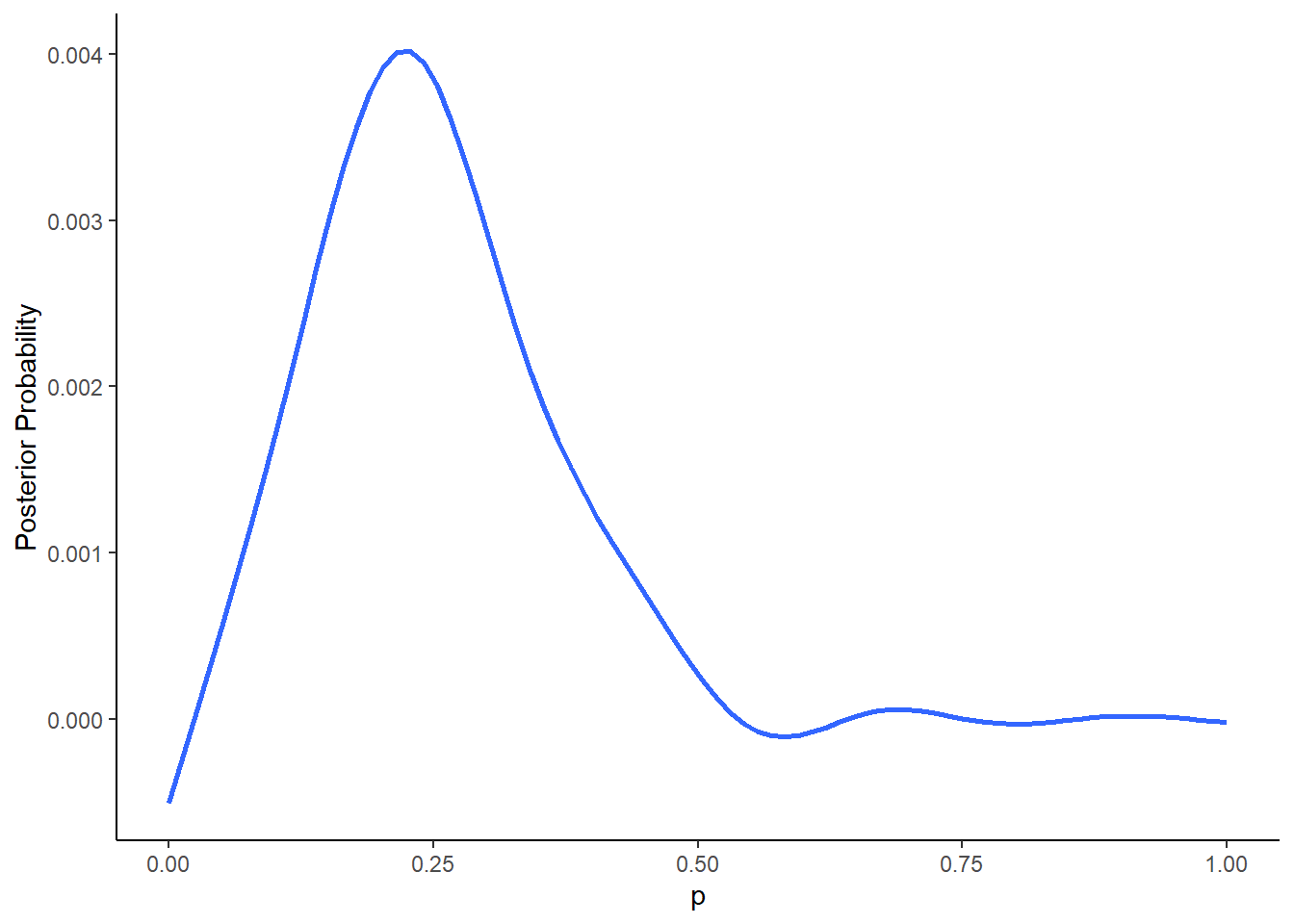

Q2

Using the posterior distribution from Q1, compute the posterior predictive distribution for the next 5 tosses of the same globe. I recommend you use the sampling method.

Sampling:

# first sample your posterior 
n <- 1e4
samples <- sample(post$poss, prob = post$post, size = n, replace = T)

# now simulate 5 tosses using the probability of each possible value 
N_toss <- 5
posterior_predict <- data.frame(probpredict = rbinom(n, size = N_toss, prob = samples))

# plot probability for each number of water samples you will get in 5 tosses
ggplot(posterior_predict) + 
  geom_bar(aes(x = probpredict)) + 
  labs(x = "Number of W Tosses") + 
  theme_classic()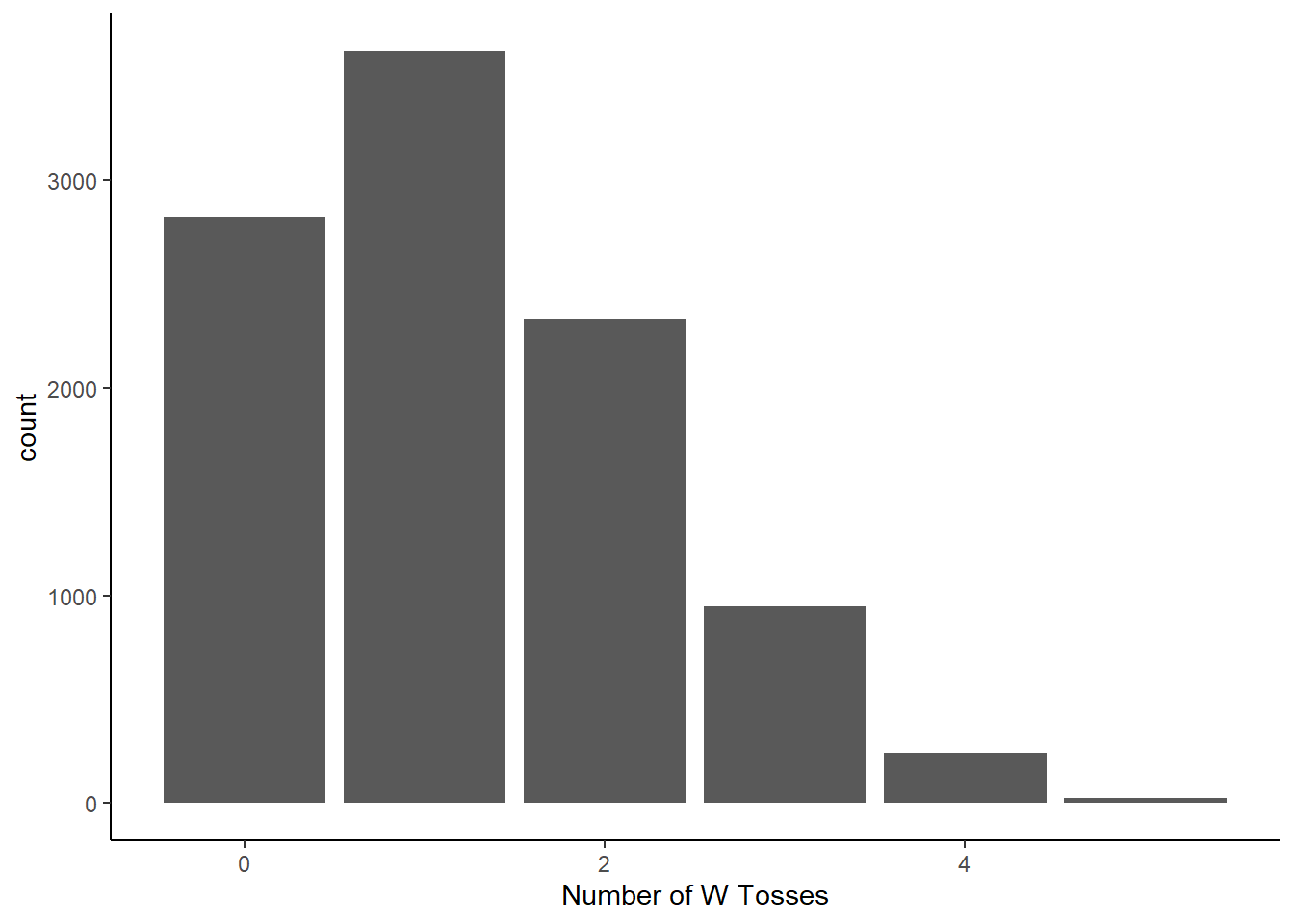

Q3 (optional):

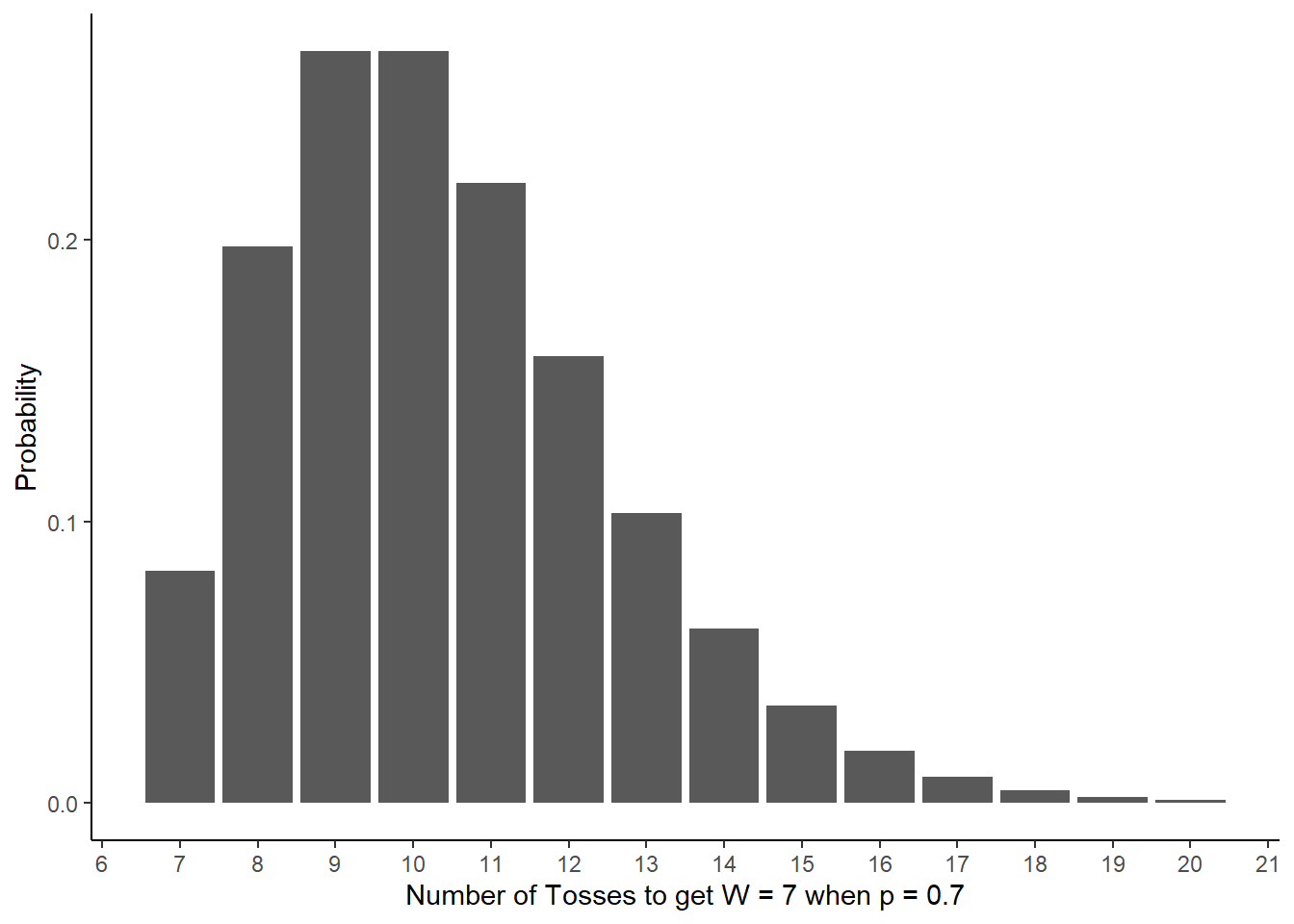
Suppose you observe W = 7 water points, but you forgot to write down how many times the globe was tossed, so you don’t know the number of land points, L. Assume that p = 0.7 and compute the posterior distribution of the number of tosses N. Hint: Use the binomial distribution.

N_tosses <- seq(7, 20)

prob_tosses <- data.frame(N_tosses = N_tosses, prob = dbinom(x = 7, size = N_tosses, prob = 0.7))

ggplot(prob_tosses) + 
  geom_col(aes(x = N_tosses, y = prob)) + 
  labs(x = "Number of Tosses to get W = 7 when p = 0.7", y = "Probability") + 
  scale_x_continuous(n.breaks = 13) + 
  theme_classic()