Lecture 05 - Elemental Confounds
Rose / Thorn
Rose: completely changed my approach to science
Thorn: why set M and not A in intervention?
Correlation
- correlation is common in nature, causation is sparse
- correlation over time series especially common
- scientific question/estimand -> recipe/estimator -> result/estimate
Association & Causation
- we must defend against confounding in our stats
- confounds mislead us - feature of the sample + how we use it
- four elemental confounds
- causes of confounds can be extremely diverse but they are all at their core made up of relationships between 3 variables
The Fork
- X and Y are associated \(Y \not\!\perp\!\!\!\perp X\) (not independent)
- Share a common cause Z
- Once stratified by Z, no association \(Y \perp\!\!\!\perp X | Z\)
dag <- dagify(
    X ~ Z,
    Y ~ Z
)

ggdag(dag) +
    theme_dag()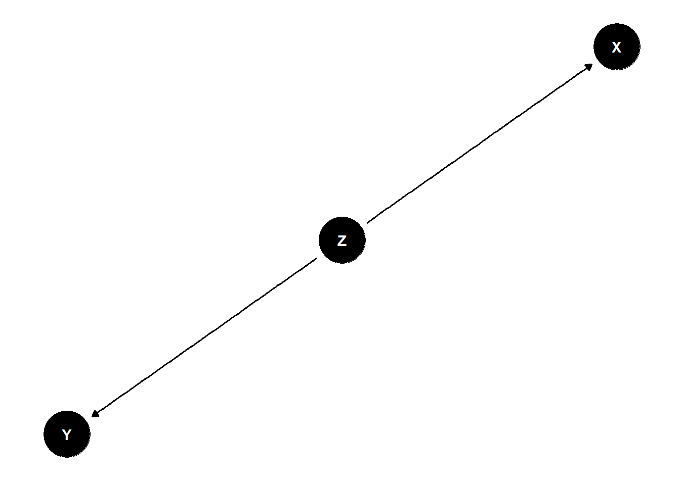
- simulation:
n <- 1000
Z <- rbern(n, 0.5)
X <- rbern(n, (1-Z)*0.01 + Z*0.9)
Y <- rbern(n, (1-Z)*0.01 + Z*0.9)

# correlated
cor(X, Y)
[1] 0.7962541# no longer correlated when we pull out Z
cor(X[Z==0], Y[Z==0])[1] -0.00895323cor(X[Z==1], Y[Z==1])[1] -0.08114448cols <- c(4,2)
n <- 300
Z <- rbern(n, 0.5)
X <- rnorm(n, (1-Z)*0.01 + Z*0.9)
Y <- rnorm(n, (1-Z)*0.01 + Z*0.9)
plot(X, Y, col=cols[Z+1]) +
abline(lm(Y[Z==1] ~ X[Z==1]), col = 2) +
abline(lm(Y[Z==0] ~X[Z==0]), col = 4) +
abline(lm(Y~ X))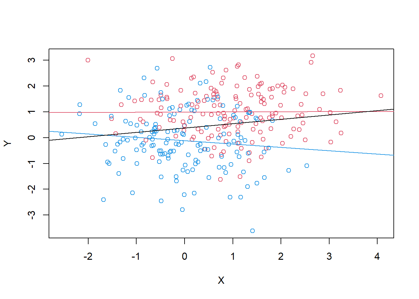
integer(0)example:
why do regions of the USA with higher rates of marriage also have higher rates of divorce?
estimand: causal effect of marriage rate on divorce rate
dag <- dagify(
    D ~ A,
    M ~ A,
    D ~ M
)

ggdag(dag) +
    theme_dag()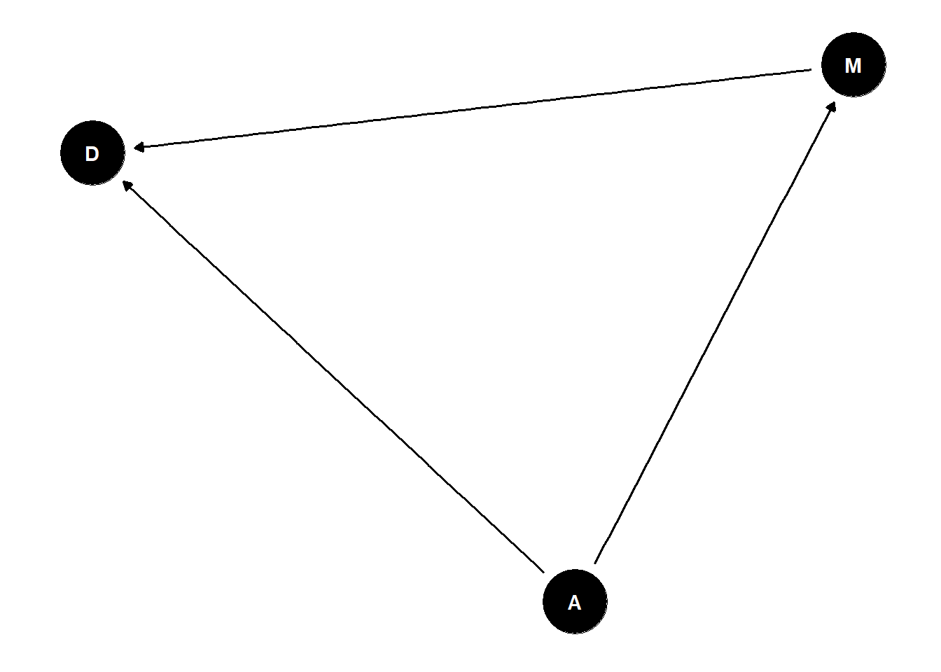
causes are not in the data
is effect of marriage rates on divorce rates just a symptom of common cause age?
need to break the fork to test direct effect – stratify by A
continuous variable stratification means that we are adding to that variable essentially to the intercept
stratifying means for every level of the stratified value, what is the association between the other two variables?
what does this mean for continuous variables?
every value of A produces a different relationship between D and M
\[ \mu_i = (\alpha + \beta_A*A) + B_D*D \]
standardizing variables is almost always helpful in linear regression
- transform measurement scales to the scale we want, as long as we remember how we changed them
- make the mean zero and divide by sd
- alpha prior is the value of average divorce rate (when standardized = 0)
- beta is within 1 and -1 for standardized variables because outside of those values the variable would be explaining all of the variation
to stratify by A, include as a term in the linear model:
\(D _i \sim Normal(\mu _i, \sigma)\)
\(\mu _i = \alpha + \beta_MM_i + \beta_AA_i\)
\(\alpha \sim Normal(0, 0.2)\)
\(\beta_M \sim Normal(0,0.5)\)
\(\beta_A \sim Normal(0, 0.5)\)
\(\sigma \sim Exponential(1)\)
library(rethinking)
data(WaffleDivorce)
d <- WaffleDivorce

# model
dat <- list(
    D = standardize(d$Divorce),
    M = standardize(d$Marriage),
    A = standardize(d$MedianAgeMarriage)
)

m_DMA <- quap(
    alist(
        D ~ dnorm(mu,sigma),
        mu <- a + bM*M + bA*A,
        a ~ dnorm(0,0.2),
        bM ~ dnorm(0,0.5),
        bA ~ dnorm(0,0.5),
        sigma ~ dexp(1)
    ) , data=dat )

plot(precis(m_DMA))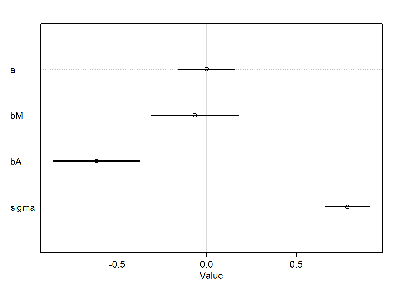
a causal effect is a manipulation of the generative model, an intervention
distribution of D when we intervene (“do”) M \(p(D|do(M))\)
- implies deleting all arrows into M and simulating D
- set values of M while holding A constant
post <- extract.samples(m_DMA)

# sample A from data
n <- 1e3
As <- sample(dat$A, size = n, replace = T)

# simulate D for M=0 (sample mean)
DM0 <- with(post, rnorm(n, a + bM*0 + bA*As, sigma))

# simulate D for M = 1 (+1 standard deviation)
# use the same A values
DM1 <- with(post, rnorm(n, a + bM*1 + bA*As, sigma))

# contrast
M10_contrast <- DM1 - DM0
dens(M10_contrast, lwd=4, col=2, xlab="effect of increase in M")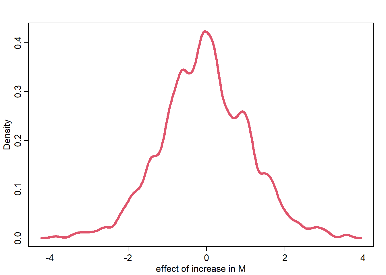
The Pipe
X and Y are associated \(Y \not\!\perp\!\!\!\perp X\)
Influence of X on Y transmitted through Z
Once stratified by Z, no association \(Y \perp\!\!\!\perp X | Z\)
dag <- dagify(
    Y ~ Z,
    Z ~ X
)

ggdag(dag) +
    theme_dag()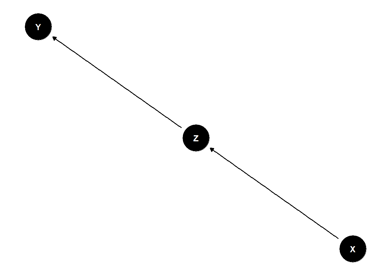
n <- 1000
X <- rbern(n, 0.5)
Z <- rbern(n, (1-X)*0.01 + X*0.9)
Y <- rbern(n, (1-Z)*0.01 + Z*0.9)
cor(X,Y)
[1] 0.7876689everything that Y knows about X, is already known by Z
- once you learn Z, there is nothing more to learn about the association
cols <- c(4,2)
n <- 300
X <- rbern(n)
Z <- rbern(n, inv_logit(X))
Y <- rbern(n, (2*Z-1))
Warning in rbinom(n, size = 1, prob = prob): NAs produced# plot- including the mediator at the wrong time can lead to incorrect inference
dag <- dagify(
   H1 ~ H0 + Treat,
   H1 ~ Fungus,
   Fungus ~ Treat

)

ggdag(dag) +
    theme_dag()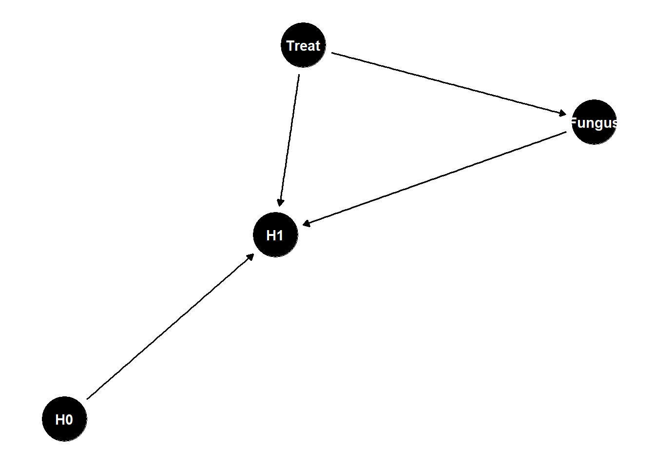
what is the total causal effect of treatment?
Treat -> Fungus -> H1 is a pipe, should not stratify by F
post-treatment bias
if you stratify by a consquence of the treatment, it can induce post-treatment bias - gives you a misleading estimate of what you’re after
consequences of treatment should not usually be included in the estimator
The Collider
X and Y are not associated (share no causes) \(Y \perp\!\!\!\perp X\)
X and Y both influence Z
Once stratified by Z, X and Y are associated \(Y \not\!\perp\!\!\!\perp X | Z\)
dag <- dagify(
    Z ~ X + Y
)

ggdag(dag) +
    theme_dag()
n <- 1000
X <- rbern(n, 0.5)
Y <- rbern(n, 0.5)
Z <- rbern(n, ifelse(X+Y>0, 0.9, 0.2))- strong correlations caused by the collider could be read as correlation but causes are not in the data
cols <- c(4,2)
N <- 300
X <- rnorm(N)
Y <- rnorm(N)
Z <- rbern(N, inv_logit(2*X+2*Y-2))

plot(X,Y, cols = cols[Z+1]) +
  abline(lm(Y[Z==1] ~ X[Z==1]), col = 2) +
  abline(lm(Y[Z==0] ~X[Z==0]), col = 4) +
  abline(lm(Y~ X))
Warning in plot.window(...): "cols" is not a graphical parameterWarning in plot.xy(xy, type, ...): "cols" is not a graphical parameterWarning in axis(side = side, at = at, labels = labels, ...): "cols" is not a
graphical parameter
Warning in axis(side = side, at = at, labels = labels, ...): "cols" is not a
graphical parameterWarning in box(...): "cols" is not a graphical parameterWarning in title(...): "cols" is not a graphical parameter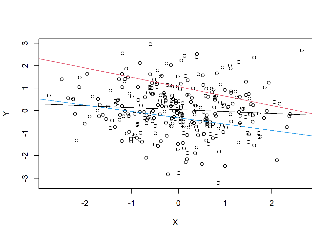
integer(0)sometimes samples come already stratified by collider
associations among the things you have measured post-selection is dangerous because the selection is often collider bias
endogenous colliders
if you include a collider in your estimator you can induce a spurious correlation
happens within your analysis
example: age and happiness
estimand: influence of age on happiness
possible confound: marital status
suppose age has zero influence on happiness, but that both age and happiness influence marital status
dag <- dagify(
   M ~ A + H
)

ggdag(dag) +
    theme_dag()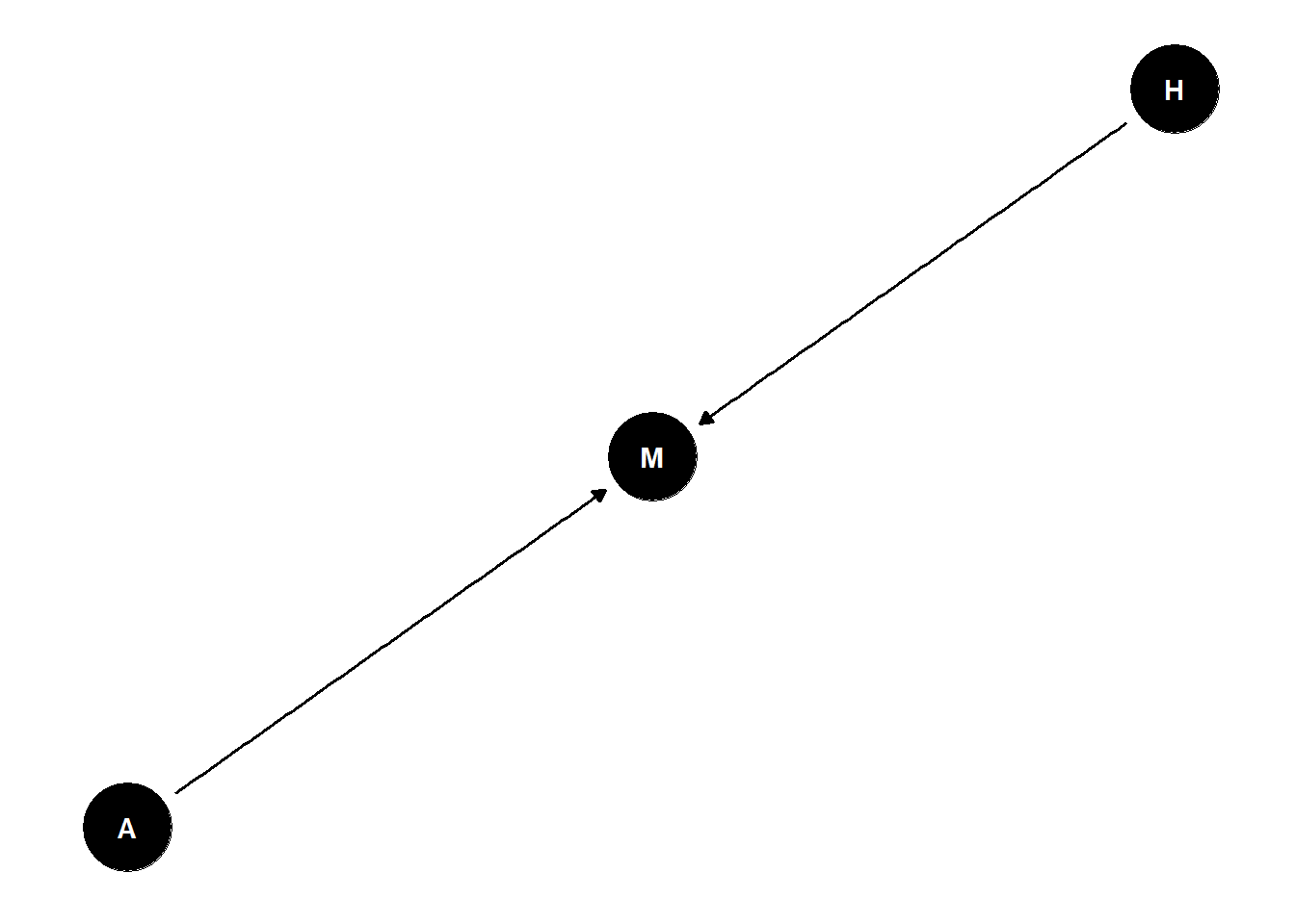
- stratified by marital status, negative association between age and happiness even though they are not related -> age/happiness are unrelated
The Descendant
how it behaves depends on what it is attached to
A is the descendant, contains information of its “parent”
X and Y are causally associated through Z \(Y \not\!\perp\!\!\!\perp X\)
A holds information about Z
Once stratified by A, X and Y less associated (if strong enough) \(Y \perp\!\!\!\perp X | A\)
dag <- dagify(
   Z ~ X,
   Y ~ Z,
   A ~ Z
)

ggdag(dag) +
    theme_dag()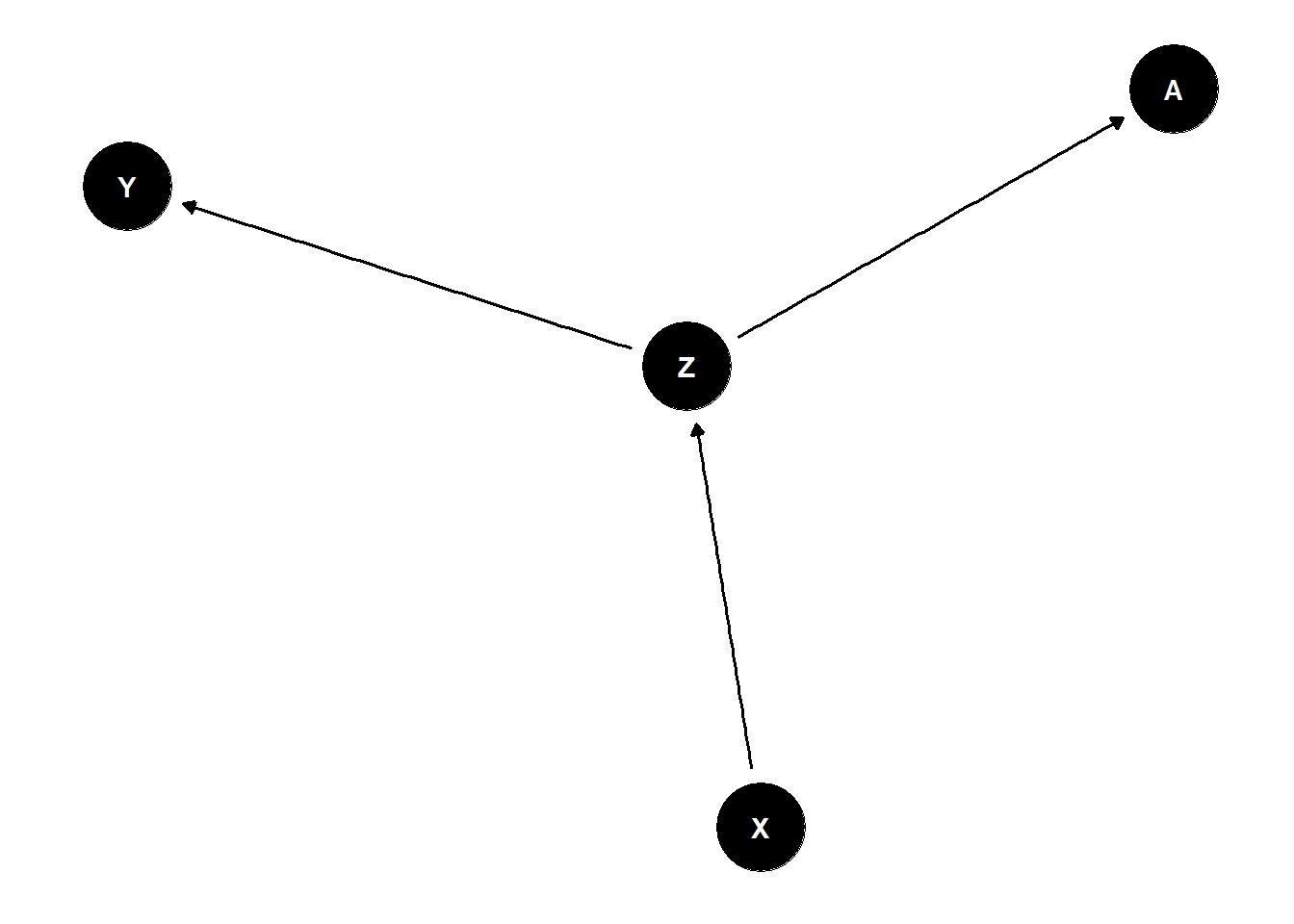
n <- 1000
x <- rbern(n, 0.5)
z <- rbern(n, (1-x)*0.1 + x*0.9)
y <- rbern(n, (1-z)*0.1 + z*0.9)
a <- rbern(n, (1-z)*0.1 + z*0.9)- descendants are everywhere - proxies