Lecture 04 - Categories & Curves

Rose / Thorn

Rose: “Unobserved causes are ignorable unless they are shared”

Thorn:

Drawing Inferences

• linear model can accomodate anything, thus we need to think carefully about our scientific model
• generative model + multiple estimands = multiple estimators
• quite often the estimate we want is not in a summary table because it depends on multiple unknowns in the posterior distribution or making assumptions about the population, so we often need to do post-processing

Categories

• categories are discrete and non-linear
• discrete, unordered types
• we want to stratify by category, to fit a separate line for each

Howell Data

Loading required package: cmdstanr

This is cmdstanr version 0.7.1

- CmdStanR documentation and vignettes: mc-stan.org/cmdstanr

- CmdStan path: C:/Users/I_RICHMO/Documents/.cmdstan/cmdstan-2.34.1

- CmdStan version: 2.34.1

Loading required package: posterior

This is posterior version 1.5.0

Attaching package: 'posterior'

The following objects are masked from 'package:stats':

    mad, sd, var

The following objects are masked from 'package:base':

    %in%, match

Loading required package: parallel

rethinking (Version 2.40)

Attaching package: 'rethinking'

The following object is masked from 'package:stats':

    rstudent

• how are height, weight, and sex causally related?
• how are height, weight, and sex statistically related?

d <- dagitty("dag {
                H -> W
                S -> W
                S -> H
             }")

drawdag(d)

• height influences weight
• sex influences weight and height
• weight is influenced by height and sex
• influence of sex is both direct and indirect on weight
• \(H = f_{H}(S)\)
• \(W = f_{W}(H,S)\)
• Unobserved causes are ignorable unless they are shared between variables (common cause) = confound

sim_HW <- function(S, b, a){
  N <- length(S)
  H <- ifelse(S==1, 150, 160) + rnorm(N, 0, 5)
  W <- a[S] + b[S]*H + rnorm(N, 0, 5)
  data.frame(S, H, W)
}

# S = 1 female : S = 2 male
S <- rbern(100)+1
dat <- sim_HW(S, b=c(0.5, 0.6), a=c(0,0))
head(dat)

  S        H         W
1 1 150.4256  70.75498
2 2 159.6225  98.62220
3 2 155.9139  96.33637
4 1 161.2995  82.11433
5 2 164.3893 109.39193
6 1 151.9171  78.64791

• scientific questions:

  • causal effect of H on W?

  • causal effect of S on W?

  • direct causal effect of S on W?

• we need to stratify by S to answer qs 2 and 3

• coding categorical variables

  • indicator variables (0/1)

  • index variables (1,2,3,4)

  • index variables are generally preferable

Index Variables

• often we want to give each index the same prior
• Influence of colour coded by: \(\alpha = [\alpha_1 , \alpha_2, \alpha_3, \alpha_4 ]\)
• \(y_i \sim Normal(\mu_i, \sigma)\)
• \(\mu_i = \alpha_{S[i]}\)
• Priors
  • \(\alpha_j \sim Normal(60, 10)\)
  • \(\sigma \sim Uniform(0, 10)\)
  • If you use indicator variables, one becomes the default and the other is the adjustment so you must set separate priors for both

Total Causal Effect of Sex on Weight

S <- rep(1, 100)
simF <- sim_HW(S, b=c(0.5, 0.6), a=c(0,0))

S <- rep(2, 100)
simM <- sim_HW(S, b=c(0.5, 0.6), a=c(0,0))

# effect of sex (male-female)
mean(simM$W - simF$W)

[1] 21.87233

• estimating model and synthetic example

S <- rbern(100)+1
dat <- sim_HW(S, b = c(0.5,0.6), a = c(0,0))

m_SW <- quap(alist(
  W ~ dnorm(mu, sigma),
  mu <- a[S],
  a[S] ~ dnorm(60, 10),
  sigma ~ dunif(0, 10)
), data = dat)

precis(m_SW, depth = 2)

           mean        sd      5.5%     94.5%
a[1]  73.937725 0.7635278 72.717460 75.157990
a[2]  94.967248 0.7950348 93.696629 96.237867
sigma  5.521365 0.3907658  4.896846  6.145885

• analyze the real sample

d <- Howell1
d <- d[ d$age >= 18,]

dat <- list(
  W = d$weight,
  S = d$male + 1
)

m_SW <- quap(alist(
  W ~ dnorm(mu, sigma), 
  mu <- a[S],
  a[S] ~ dnorm(60, 10),
  sigma ~ dunif(0, 10)
), data = dat)

• posterior means and predictions
• a1 and a2 are often not what we are after
  • difference in mean weight is not in the posterior - must calculate a contrast
  • but the mean weight of each category does exist in the posterior
• first plot is just mean weight for each sex
• distributions of weights is the posterior predicted, second figure
• contrast is usually what we are after, third figure

# posterior mean W
post <- extract.samples(m_SW)
density_f <- density(post$a[, 1])
density_m <- density(post$a[, 2])
plot(density_f, col=2, xlim = c(min(density_f$x,density_m$x), max(density_f$x,density_m$x)), main = "Posterior Mean Weight (kg)") + 
lines(density_m, col=4)

integer(0)

# posterior W predictions
W1 <- rnorm(1000, post$a[,1], post$sigma)
W2 <- rnorm(1000, post$a[,2], post$sigma)
predict_f <- density(W1)
predict_m <- density(W2)
plot(predict_f, col=2, xlim = c(min(predict_f$x,predict_m$x), max(predict_f$x,predict_m$x)), main = "Posterior Predicted Weight (kg)") + 
lines(predict_m, col=4)

integer(0)

• contrasting

  • need to compute the difference between the categories

  • it is not legitimate to compare overlap in distributions

  • we must compute contrast distribution

  • overlap in distributions does not indicate that they are the same (or different)

• average difference between men and women in this sample:

mu_contrast <- post$a[,2] - post$a[,1]
dens(mu_contrast)

• weight contrasting:

# contrast
W_contrast <- W2 - W1
dens(W_contrast)

# proportion above zero
sum(W_contrast > 0)/1000

[1] 0.801

sum(W_contrast < 0)/1000

[1] 0.199

Direct Causal Effect of Sex on Weight

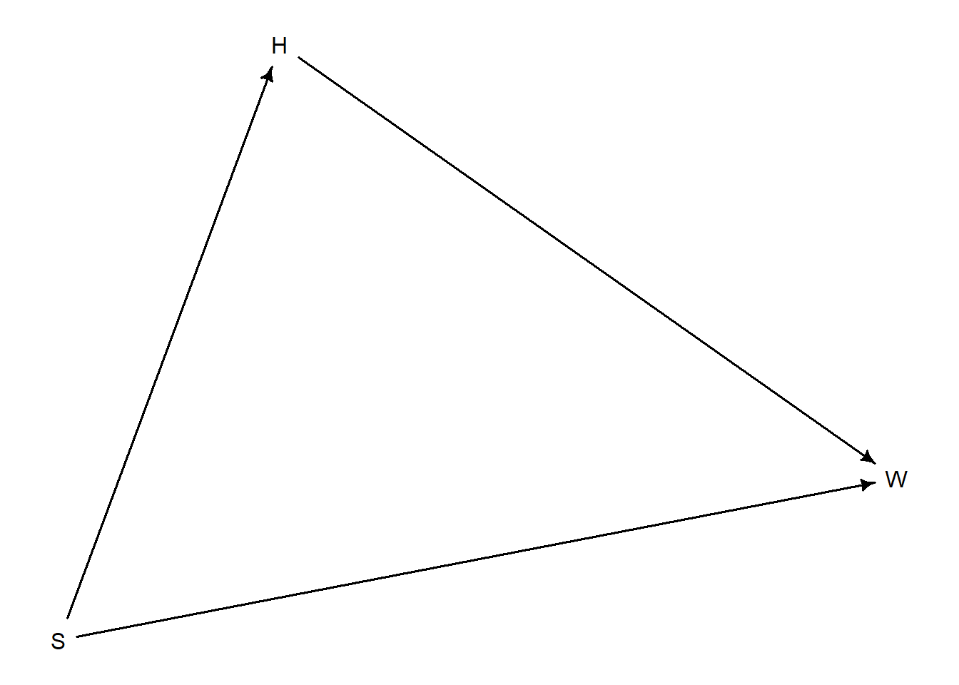
• “controlling” for the indirect effect of sex through height
• want to “block” association through H

S <- rbern(100)+1
# slopes are the same so there is no effect of height on weight through slope but men are on average 10 kg heavier (intercept 10)
set.seed(12)
dat <- sim_HW(S, b = c(0.5, 0.5), a = c(0, 10))

• \(W_{i} \sim Normal(\mu _{i}, \sigma)\)

• \(\mu _{i} = \alpha _{S[i]} + \beta _{S[i]}(H_{i} - \bar H)\)

  • This equation centers the height \((H_{i} - \bar H)\)

  • Centering H means that alpha represents the average weight of a person with average height

  • Centering also makes priors easier for alpha

  • \(\alpha = [\alpha _{1}, \alpha _{2}]\) , \(\beta = [\beta _{1}, \beta _{2}]\)

• analyze the sample

d <- Howell1
d <- d[d$age >= 18, ]
dat <- list(W = d$weight, H = d$height, Hbar = mean(d$height), S = d$male + 1)

m_SHW <- quap(alist(
  W ~ dnorm(mu, sigma),
  mu <- a[S] + b[S]*(H-Hbar),
  a[S] ~ dnorm(60, 10),
  b[S] ~ dunif(0, 1),
  sigma ~ dunif(0, 10)
), data = dat)

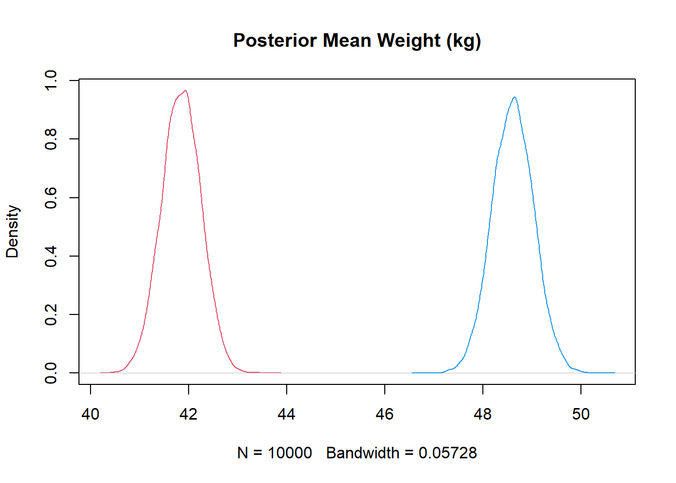
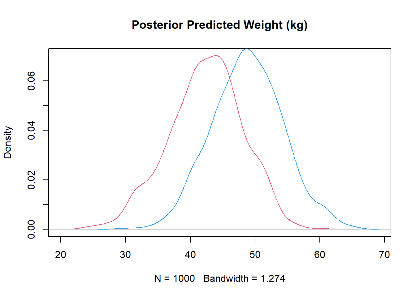
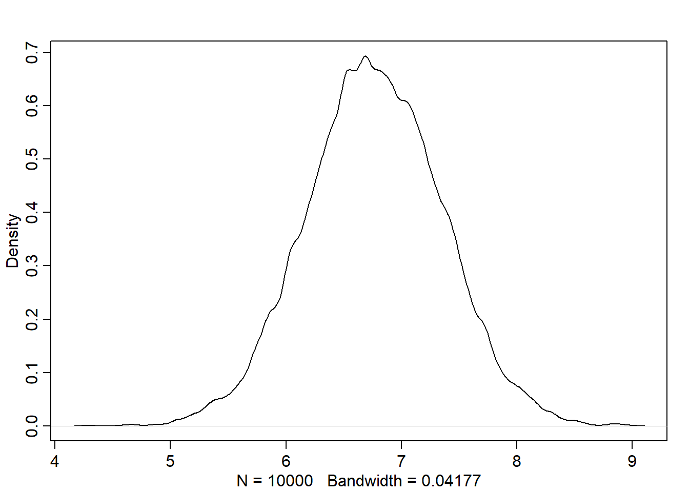
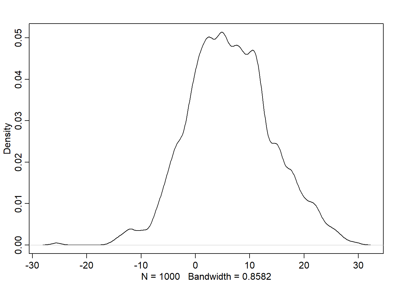
• we need to compute the difference of expected weight at each height to get the actual estimate that we are looking for (for the direct effect of sex on weight)
• compute posterior predictive for each group, calculate contrast, plot

xseq <- seq(from=130, to=190, len=50)

muF <- link(m_SHW, data = list(S=rep(1,50), H=xseq, Hbar=mean(d$height)))

muM <- link(m_SHW, data = list(S=rep(2,50), H=xseq, Hbar = mean(d$height)))

mu_contrast <- muF - muM

plot(NULL, xlim=range(xseq), ylim = range(-6, 8), xlab = "height (cm)", ylab = "weight contrast (F-M)") +
lines(xseq, apply(muF, 2, mean)) + 
lines(xseq, apply(muM, 2, mean)) 

integer(0)

#for (p in c(0.5, 0.6, 0.7, 0.8, 0.9, 0.99)) {
#  shade(apply(mu_contrast, 2, PI, prob = p), xseq)
#  abline(h=0)
#  }

• women tend to be heavier at high heights and vice versa for men

• but most of the effect is centered around zero, therefore:

• nearly all of the causal effects of S acts through H

  • when we block H, we see very little effect of sex on weight

Categorical Variables

• common, easy to use with index coding

• use samples to compute relevant contrasts

• always summarize (mean, interval) as the last step

• we want mean difference and not difference of means

Curves from Lines

• many non linear relationships, which can be fit my linear models easily (but not mechanistic, like a geocentric model)

• linear models can easily fit curves: 2 strategies

  • polynomials (bad)

  • splines and GAMs (less bad + useful)

Polynomial Models

• still linear because its an additive function of the parameters

• create strange symmetries and explosive uncertainty

• no local smoothing, only global smoothing

• any data point at any part of the x-axis can significantly change the curve even at arbitrarily far distances

• can’t predict anything outside of the data with any certainty

• do not use

Splines + GAMs

• great for locally inferred function

• add together a bunch of locally trained terms

• can add as many locally trained terms as you want

• each term has a weight and slope and only affects its own region

Full Luxury Bayes

• instead of two models for two estimands, use one model for full causal model
• can simulate interventions with this approach
• requires more simulations

m_SHW_full <- quap(alist(
  
  # weight
  W ~ dnorm(mu, sigma),
  mu <- a[S] + b[S]*(H-Hbar),
  a[S] ~ dnorm(60, 10),
  b[S] ~ dunif(0, 1),
  sigma ~ dunif(0, 10),
  
  # height
  H ~ dnorm(nu, tau),
  nu <- h[S],
  h[S] ~ dnorm(160, 10),
  tau ~ dunif(0, 10)
  
), data = dat)


post <- extract.samples(m_SHW_full)
Hbar <- dat$Hbar
n <- 1e4

#with(post, {
#  
#  H_S1 <- rnorm(n, h[,1], tau)
#  W_S1 <- rnorm(n, a[,2] + b[,1]*(H_S2-Hbar), sigma)
#  
#  W_do_S <<- W_S2 - W_S1
#  
#})
#
## automate
#HWsim <- sim(m_SHW_full, data = list(S=c(1,2)), vars = c("H", "W"))
#W_do_S_auto <- HWsim$W[,2] - HWsim$W[,1]

• you can either do one statistical model for each estimand OR one simulation for each estimand (full luxury Bayes)

TODO: