Homework - Week 02
Q1
From the Howell1 dataset, consider only the people younger than 13 years old. Estimate the causal association between age and weight. Assume that age influences weight through two paths. First, age influences height. Second, age directly influences weight through age-related changes in muscle growth and body proportions. Draw the DAG that represents these causal relationships. And then write a generative simulation that takes age as an input and simulates height and weight, obeying the relationships in the DAG.
DAG:
dagified <- dagify(
    # outline relationships between your variables
    Weight ~ Age + Height,
    Height ~ Age,
   # assign exposure and outcome
    exposure = 'Age',
    outcome = 'Weight',
   # assign coordinates so they aren't randomly assigned
    coords = list(x = c(Age = -1, Height = 0, Weight = 0),
                  y = c(Age = 0, Height = 1, Weight = -1))) %>%
    # tidy_dagitty makes dag into tidy table format
    tidy_dagitty() %>%
    # add column that assigns variables to groups that you want to colour code
    mutate(status = case_when(name == "Age" ~ 'exposure',
                              name == "Weight" ~ 'outcome',
                              .default = 'NA'))

  ggplot(dagified, aes(x = x, y = y, xend = xend, yend = yend)) +
    theme_dag() +
    # colour nodes by the column you made in previous step
    geom_dag_point(aes(color = status)) +
    # add labels so you can have more readable variable names
    geom_dag_label_repel(aes(label = name, fill = status),
                         color = "white", fontface = "bold") +
    # adding geom_dag_edges here so that the arrows will go over the labels
    geom_dag_edges() +
    # assign the colours that you want
    scale_fill_manual(values = c('darkseagreen', 'grey', 'lightblue')) +
    scale_colour_manual(values = c('darkseagreen', 'grey', 'lightblue')) +
   # removing colour legend here
    theme(legend.position = 'none')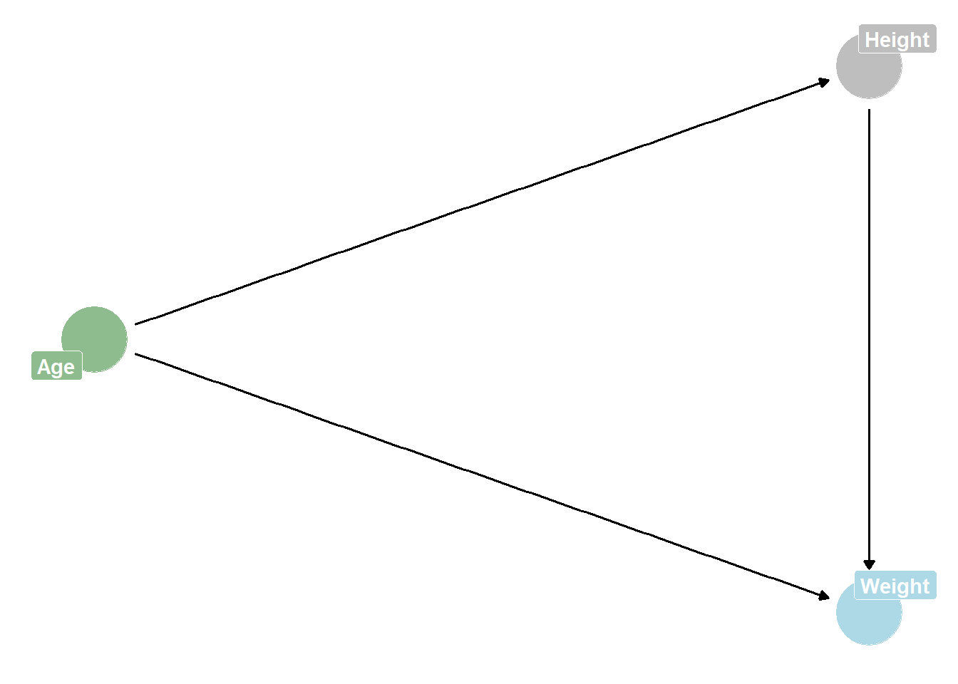
- \[ Weight = f_{Weight}(Age, Height) \]
Generative Simulation:
N <- 1e3

# generate 1000 youth ranging from 1-12
age <- sample(seq(from = 1, to = 12), size = N, replace = T)

# generate heights that are variable but increase with increasing age
# height is 8 * age with 2 SD (maybe too small for babies but generally okay)
bAH <- 8
height <- rnorm(N, bAH*age, 2)

# generate weights that are variable but increase with increasing height and age (but are smaller than heights)
bAW <- 0.1
bHW <- 0.5
weight <- rnorm(N, bAW*age + bHW*height, 2)

gen <- data.frame(age, height, weight)

head(gen)
age height weight
1 9 70.97997 35.98964
2 6 46.53393 23.45612
3 10 80.79248 40.95918
4 10 81.19892 40.68226
5 7 55.24166 30.09088
6 12 93.72050 49.41547Q2
Estimate the total causal effect of each year of growth on weight.
- Total causal effect does not stratify by height, it includes both direct and indirect effects
Prior predictive:
tar_load(h02_mAW_prior)
print(h02_mAW_prior$formula)
weight ~ age prior_summary(h02_mAW_prior) prior class coef group resp dpar nlpar lb ub source
uniform(0, 10) b user
uniform(0, 10) b age (vectorized)
normal(35, 2) Intercept user
exponential(1) sigma 0 usergen_sub <- gen %>% select(c(age))
epred <- add_epred_draws(gen_sub, h02_mAW_prior, ndraws = 100)
ggplot(epred, aes(x = age, y = .epred)) +
geom_line(aes(group=.draw), alpha = 0.1) +
labs(y = "Predicted Weight", x = "Age") +
theme_classic()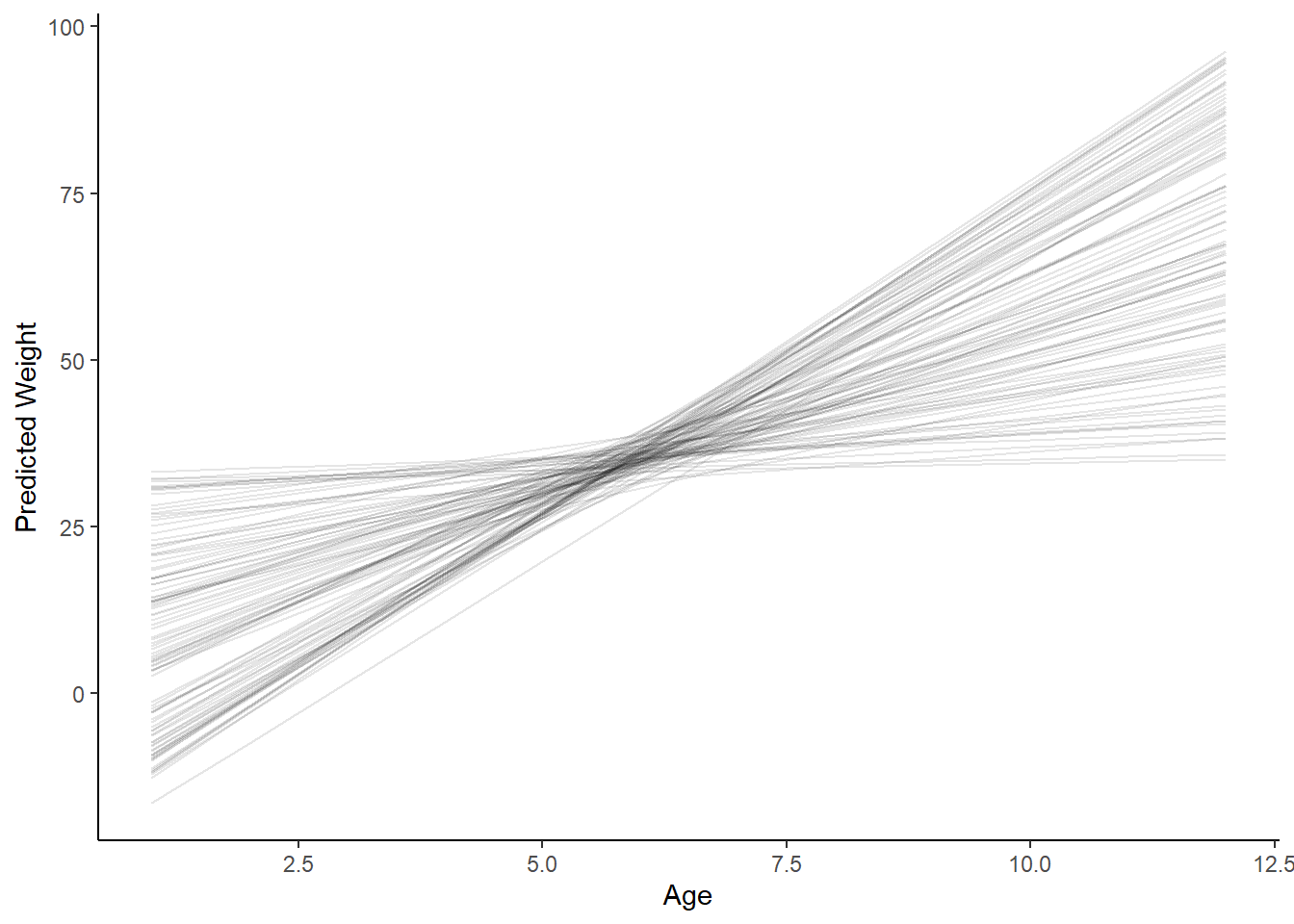
Posterior Distribution:
tar_load(h02_mAW)
print(h02_mAW$formula)
weight ~ age data(Howell1)
youth <- Howell1 %>% filter(age < 13)
avg_youth <- youth %>%
summarize(age = mean(age))
pred_mean <- h02_mAW %>%
epred_draws(newdata = avg_youth)
ggplot(pred_mean, aes(x = .epred)) +
stat_halfeye() +
labs(x = "Weight (kg) for kid of average age", y = "") +
theme_classic() 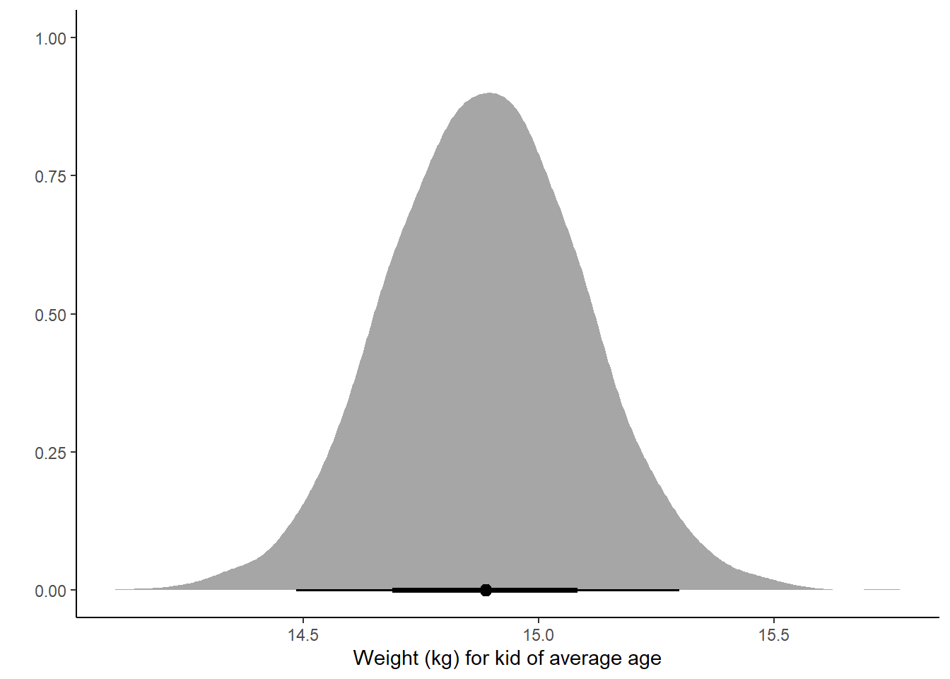
# prediction for relationship between age and weight
epred <- h02_mAW %>%
      epred_draws(youth)

# plot slopes
ggplot(data = youth, aes(x = age)) +
  stat_lineribbon(aes(x = age, y = .epred), data = epred) +
  geom_jitter(aes(y = weight), width = .1, height = 0, alpha = 0.7) +
  scale_fill_brewer(palette = "Greys") +
  labs(y = 'Linear Model Predicted Weight (kg)', x = "Age (yrs)", fill = "Credible Interval") +
  theme_classic()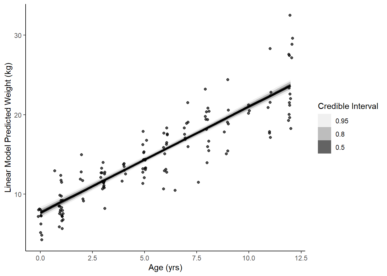
Posterior Predictive:
# prediction for average kid
pred_mean <- h02_mAW %>%
  predicted_draws(newdata = avg_youth)


ggplot(pred_mean, aes(x = .prediction)) +
  stat_halfeye() +
  labs(x = "Weight (kg) for kid of average age", y = "") +
theme_classic() 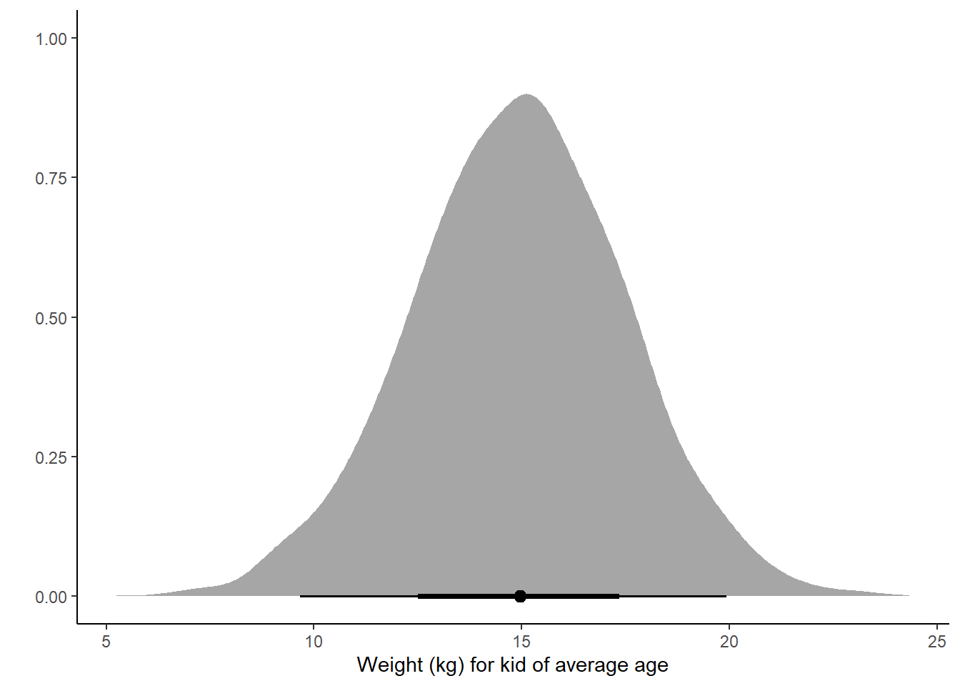
# prediction for relationship between age and weight
pred <- h02_mAW %>%
      predicted_draws(youth)

# plot slopes
ggplot(data = youth, aes(x = age)) +
  stat_lineribbon(aes(x = age, y = .prediction), data = pred) +
  geom_jitter(aes(y = weight), width = .1, height = 0, alpha = 0.7) +
  scale_fill_brewer(palette = "Greys") +
  labs(y = 'Predicted Weight (kg)', x = "Age (yrs)", fill = "Credible Interval") +
  theme_classic()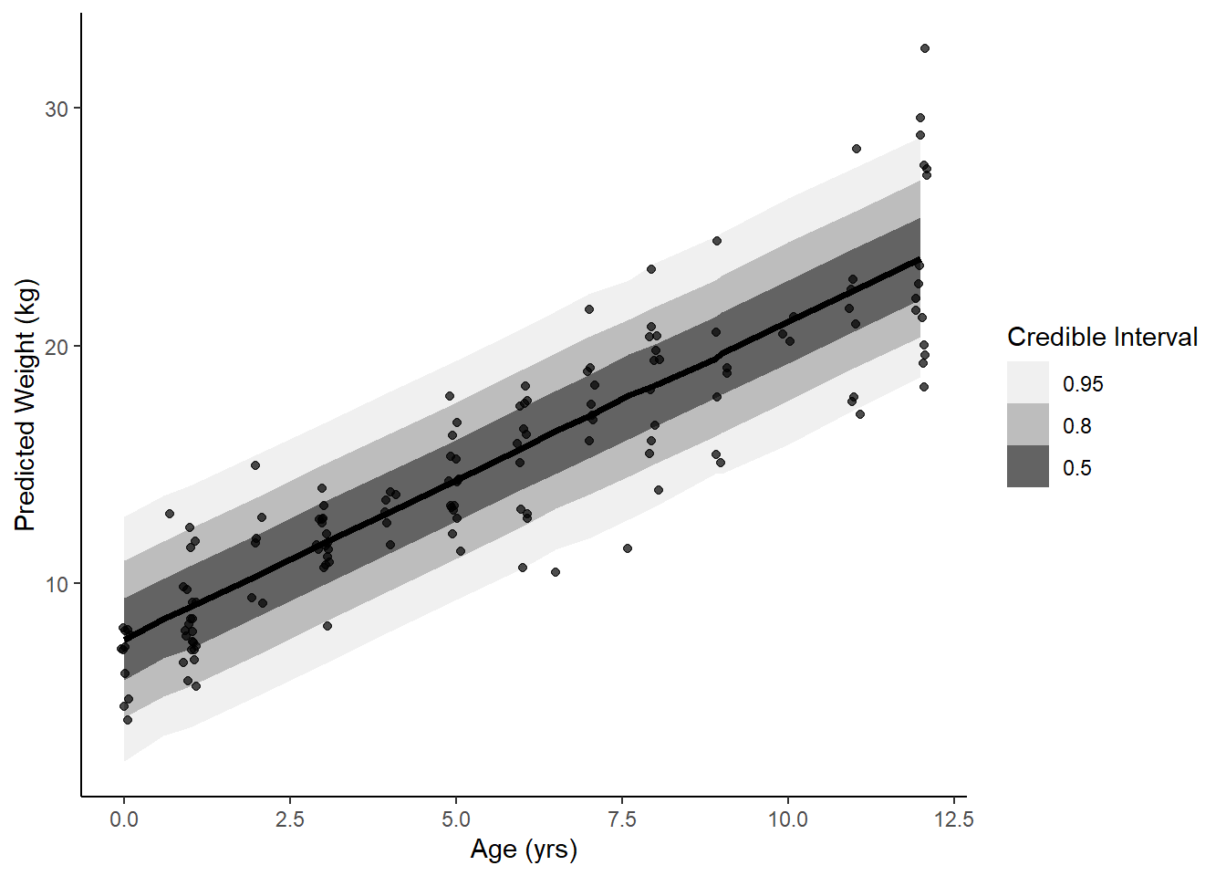
Q3 (optional):
The data in
data(Oxboys)(rethinkingpackage) are growth records for 26 boys measured over 9 periods. I want you to model their growth. Specifically, model the increments in growth from one period (Occassion in the data table) to the next. Each increment is simply the difference between height in one occasion and height in the previous occasion. Since none of these boys shrunk during the study, all of the growth increments are greater than zero. Estimate the posterior distribution of these increments. Constrain the distribution so it is always positive - it should not be possible for the model to think that boys can shrink from year to year. Finally compute the posterior distribution of the total growth over all 9 occasions.
- \[Growth = f(Time)\]
- where Growth = \[\Delta Height\]
- and Time = Occasion
- \[ \Delta Height = f(Occasion) \]
Check that our priors are constrained to positive values:
data(Oxboys)

ox <- Oxboys %>%
  group_by(Subject) %>%
  mutate(growth = height - lag(height, default = first(height), order_by = Occasion)) %>%
  # remove first occasion because there is no growth
  filter(Occasion != 1)

tar_load(h02_mGO_prior)
prior_summary(h02_mGO_prior)
prior class coef group resp dpar nlpar lb ub source
normal(1.6, 0.5) Intercept 0 user
exponential(1) sigma 0 userposprior <- add_epred_draws(ox, h02_mGO_prior, ndraws = 100)
ggplot(posprior, aes(x = .epred)) +
geom_histogram() +
labs(x = "Intercept")+
theme_classic()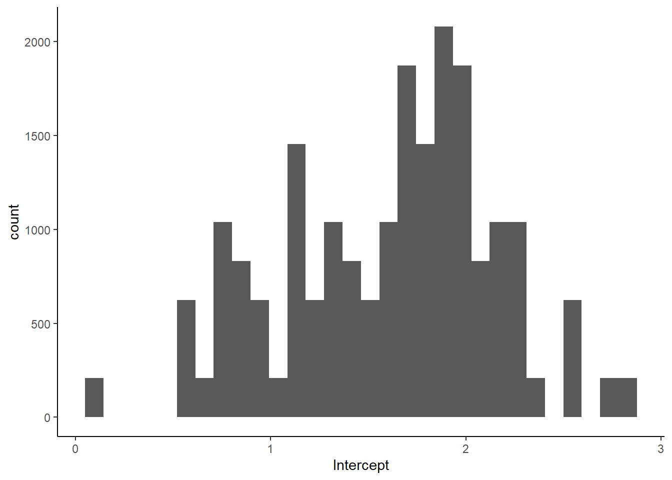
Success! We see no negative intercept values in our prior.
Investigate posterior distribution:
tar_load(h02_mGO)
h02_mGO$formula
growth ~ 1 post_growth <- h02_mGO %>%
predicted_draws(newdata = ox)
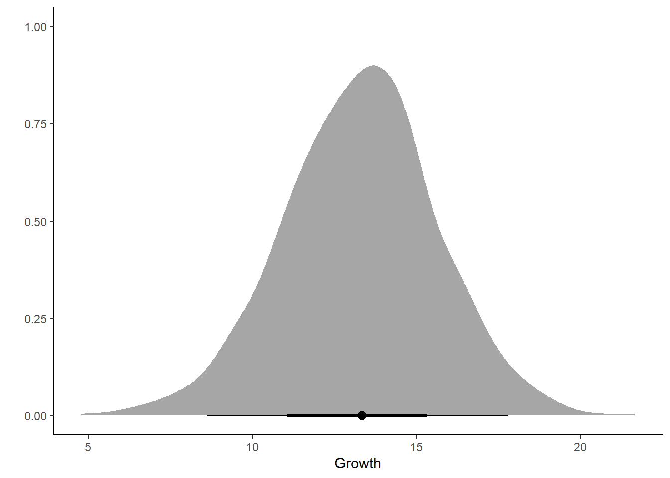
ggplot(post_growth, aes(x = .prediction)) +
stat_halfeye() +
labs(x = "Growth", y = "") +
theme_classic() 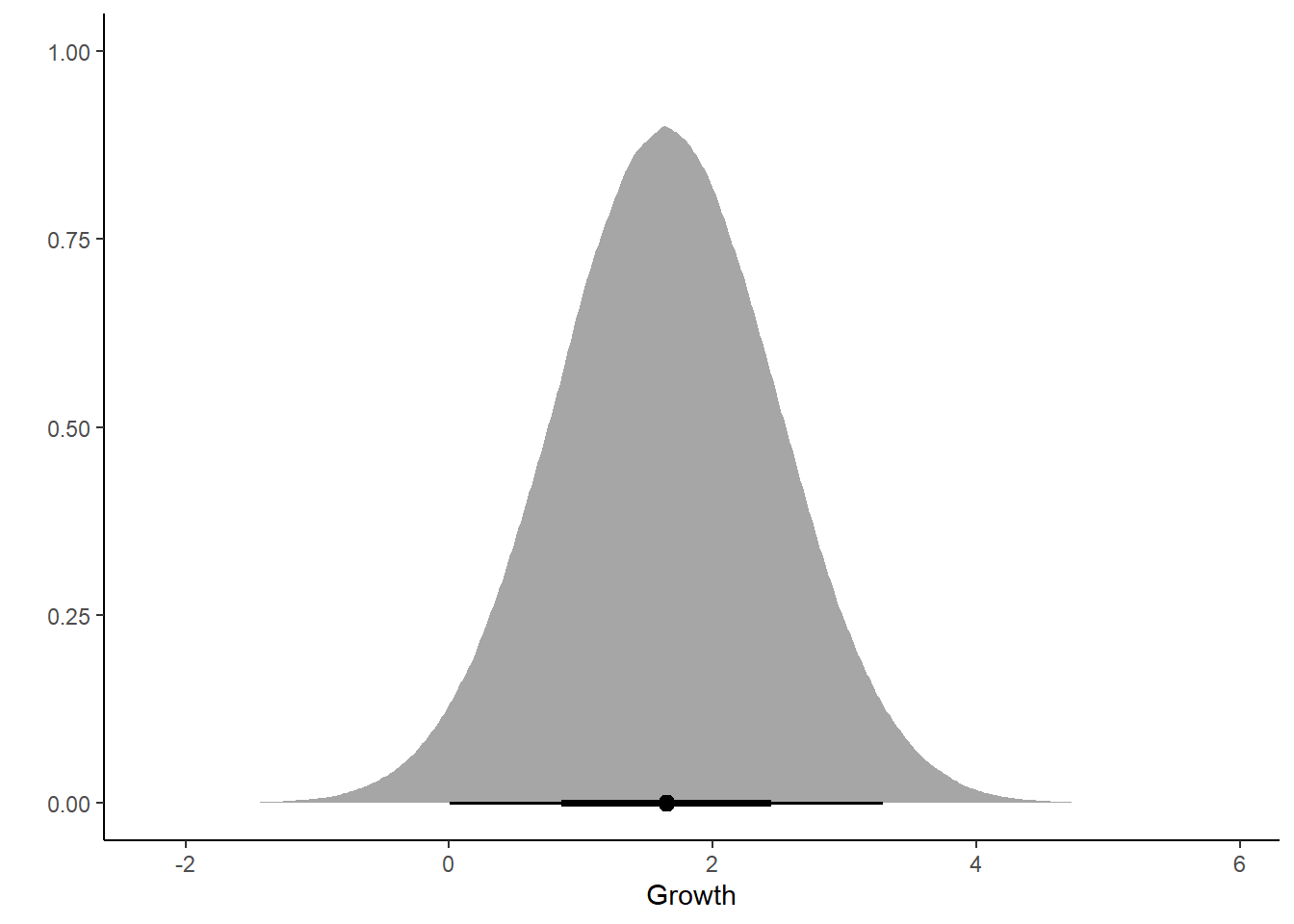
Hmm… maybe not a success …
Total growth over 8 occasions:
# need to randomly sample the posterior 8 times and then sum the samples, 1000 times

t <- data.frame(total_growth = replicate(1000, {sum(sample(post_growth$.prediction, 8, replace = T))}))

ggplot(t, aes(x = total_growth)) +
  stat_halfeye() +
  labs(x = "Growth", y = "") +
  theme_classic()