Lecture 03 - Geocentric Models

Author

Isabella C. Richmond

Published

February 8, 2023

Rose / Thorn

Rose: Non-independent variables in a summary table

Thorn: Stupid resolution to my plot coding issue

Linear Regressions

essentially a geocentric model - overly simplified
separate from a causal model
associations are from the causal model, not the statistical model

Gaussian Distributions

there are many more ways to end up in the center than to end up on the periphery
why the Gaussian distribution spontaneously occurs in natural systems
generative: if we add fluctuations, we tend towards normal distribution (lots of summed fluctuations in nature)
inferential: estimating mean and variance, normal distribution is best one to use because it is least informative (no other information present)
normal distribution is just a tool for estimating mean/variance because it has widest distribution
- data doesn’t have to be normal to be able to leverage the tool to estimate mean/variance

Workflow

State a clear question
Sketch causal assumptions
Define generative model from sketch
Use generative model to build estimator
Profit

library(rethinking)
library(dagitty)
data(Howell1)

Describing Models

= is deterministic

~ is distributional

Howell Example

Question/Estimand: Describe association between adult weight and height

d2 <- Howell1[Howell1$age>=18,]

Scientific model: weight is some function of height and unobserved influences

d <- dagitty("dag {
                H -> W
                U -> W
             }")

drawdag(d)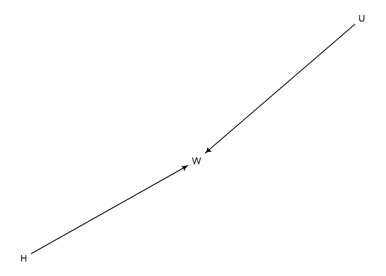

\[ W = f(H, U) \]

Generative/Statistical model

Two options: dynamic (complex and ongoing) and static
- Static model allows us to imagine changes at specific times and still use a Gaussian distribution
For adults, weight is a proportion of height plus the influence of unobserved causes

\[ W = \beta H+U \]

sim_weight <- function(H, b, sd){
  U <- rnorm(length(H), 0, sd)
  W <- b*H + U
  return(W)
}

H <- runif(200, min = 130, max = 170)
W <- sim_weight(H, b = 0.5, sd = 5)
plot(W ~ H, col = 2, lwd = 3)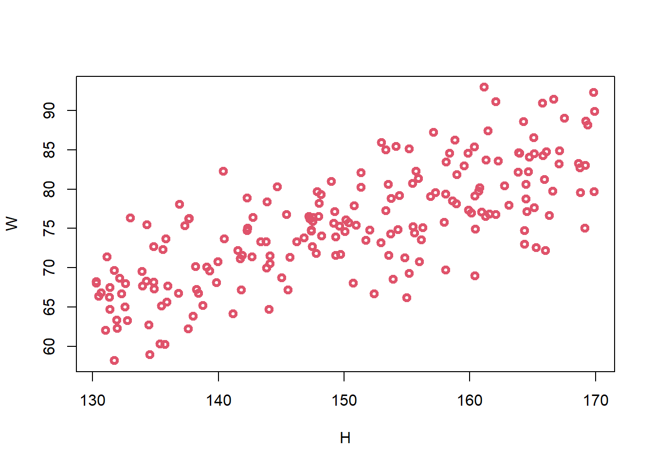

can adjust to produce biologically unrealistic relationships by adjusting b to be large or small

\[ W_i = \beta H_i + U_i \\ U_i \sim Normal(0, \sigma) \\ H_i \sim Uniform(130, 170) \]

~ indicates distribution
= is deterministic
we want to estimate how the average weight changes with height

\[ E(W_{i}|H_{i}) = \alpha + \beta H_{i} \]
\(E(W_{i}|H_{i})\) = average weight conditional on height
\(\alpha\) = intercept (when height is 0, what is weight? Scientifically should be zero but putting it in model to make sure our model is scientifically sound)
\(\beta\) = slope
Posterior distribution:
- \[ Pr(\alpha,\beta,\sigma| H_{i}, W_{i}) = \frac{Pr(W_{i}|H_{i}, \alpha,\beta,\sigma)Pr(\alpha,\beta,\sigma)}{Z} \]
- alpha, beta, sigma are our three unknowns: alpha and beta define the line and sigma defines the error around it
- unknowns are conditional (|) on the data H_i and W_i
- alpha, sigma, beta are unknown so we need a posterior distribution for them (and they are dependent on the data)
- \(Pr(\alpha,\beta,\sigma| H_{i}, W_{i})\) = posterior probability of specific line
- \(Pr(W_{i}|H_{i}, \alpha,\beta,\sigma)\) = probability of each weight dependent on height value, alpha, beta, sigma (garden of forking data)
- \(Pr(\alpha,\beta,\sigma)\) = prior
- Z = normalizing constant
- \(W_{i} \sim Normal(\mu _{i}), \sigma)\): linear model
- \(\mu _{i} = \alpha + \beta H_{i}\)
Quadratic approximation (continuous version of grid approximation)
- approximate posterior distribution as a multivariate Gaussian distrubution
- posteriors are often Gaussian
- \(W_{i} \sim Normal(\mu _{i}), \sigma)\)
- \(\mu _{i} = \alpha + \beta H_{i}\)
- \(\alpha \sim Normal(0,10)\)
- \(\beta \sim Uniform(0,1)\)
- \(\sigma \sim Uniform(0, 10)\)

H <- runif(10, 130, 170)
W <- sim_weight(H, b = 0.5, sd = 5)

m3.1 <- quap(alist(
  W ~ dnorm(mu, sigma),
  mu <- a + b*H,
  a ~ dnorm(0, 10),
  b ~ dunif(0, 1),
  sigma ~ dunif(0, 10)
), data = list(W=W, H=H))

Priors
- we want to constrain to scientifically plausible values
- justify with information outside the data - like the rest of model
- priors have no essential differences from posteriors except for data – we can use them as generative models and ensure that our assumptions are reasonable

n <- 1e3
a <- rnorm(n, 0, 10)
b <- runif(n, 0, 1)
plot(NULL, xlim = c(130, 170), ylim = c(50, 90)) + 
for (j in 1:50) abline(a=a[j], b=b[j], col = 'red')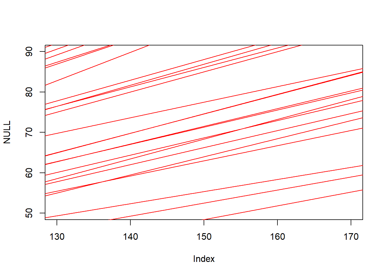

integer(0)

Validate model

test statistical model with simulated observations from scientific model - need to test if your model is working
use many values and make sure your model responds appropriately

# model summary
precis(m3.1)

           mean         sd        5.5%      94.5%
a     0.6093014 9.50424778 -14.5803222 15.7989250
b     0.5045905 0.06551189   0.3998898  0.6092911
sigma 6.1344656 1.35444780   3.9697964  8.2991347

Analyze data

dat <- list(W = d2$weight, H = d2$height)
m3.2 <- quap(alist(
  W ~ dnorm(mu, sigma),
  mu <- a + b*H,
  a ~ dnorm(0, 10), 
  b ~ dunif(0, 1),
  sigma ~ dunif(0, 10)
), data = dat)

precis(m3.2)

             mean         sd       5.5%       94.5%
a     -43.7106844 4.17274593 -50.379538 -37.0418305
b       0.5738951 0.02696368   0.530802   0.6169883
sigma   4.2584569 0.16227623   3.999108   4.5178056

parameters are not independent of one another, they cannot be independently interpreted
- use posterior predictions and describe/interpret those by sampling the posterior distribution
Posterior Predictive Distribution

post <- extract.samples(m3.2)
plot(d2$height, d2$weight) + 
for (j in 1:20) abline(a=post$a[j], b=post$b[j])

integer(0)

height_seq <- seq(130, 190, len = 20)
W_postpred <- sim(m3.2, data = list(H=height_seq))
W_PI <- apply(W_postpred, 2, PI)

plot(d2$height, d2$weight) + 
for (j in 1:20) abline(a=post$a[j], b=post$b[j]) +
lines(height_seq, W_PI[1,], lty = 2) +
lines(height_seq, W_PI[2,], lty = 2)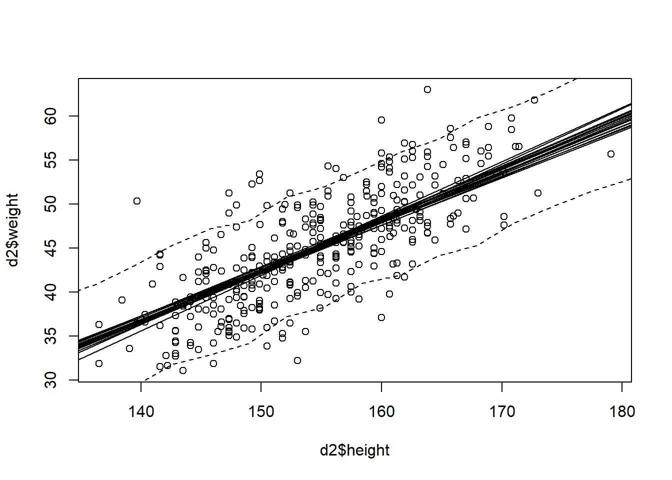

integer(0)