Rose / Thorn
Rose: understanding the predictive posterior this time
Thorn: what if you don’t know your misclassification rate
Globe Example
estimand: proportion of the globe covered in water - do people know what an estimand is?
a research/scientific question
estimator : statistical way of producing an estimate
generative model tests your estimator
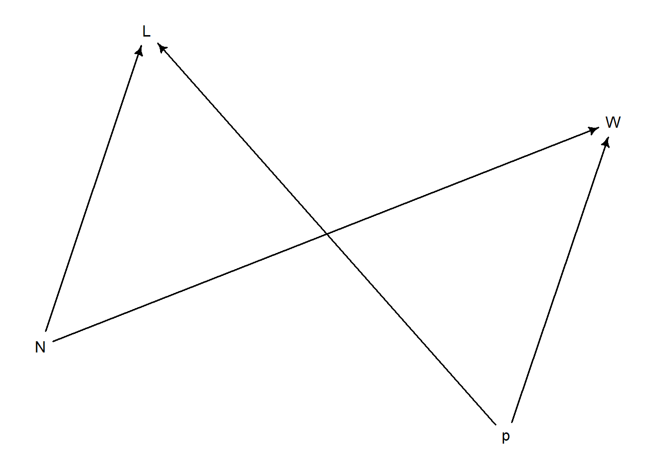
Generative Model (globe)
p = proportion of waterW = water observations
N = number of tosses
L = land observations
N influences W and L because higher tosses means higher numbers
start with how the variables influence each other, i.e., causal model
start conceptually, with science
intervention on N is also an intervention on W and L
library (dagitty)library (rethinking)
Loading required package: cmdstanr
This is cmdstanr version 0.7.1
- CmdStanR documentation and vignettes: mc-stan.org/cmdstanr
- CmdStan path: C:/Users/I_RICHMO/Documents/.cmdstan/cmdstan-2.34.1
- CmdStan version: 2.34.1
Loading required package: posterior
This is posterior version 1.5.0
Attaching package: 'posterior'
The following objects are masked from 'package:stats':

    mad, sd, var
The following objects are masked from 'package:base':

    %in%, match
Loading required package: parallel
rethinking (Version 2.40)
Attaching package: 'rethinking'
The following object is masked from 'package:stats':

    rstudent
<- dagitty ("dag { p -> W p -> L N -> W N -> L }" )drawdag (d)
\[
W,L = f(p,N)
\]
W and L are functions of p and N
DAGs are not generative, but they make causal models which allow us to make generative models
they represent functional relationships
Bayesian Data Analysis
For each possible explanation of the sample,
count all the ways the sample could happen (given a particular explanation)
explanations with more ways to produce the sample are more plausible
Garden of Forking Data
relies on samples being independent
relative differences between probabilities are dependent on sample size (differences will be smaller with smaller sample sizes because there is less evidence)
normalizing to probability allows for interpretability and easier math
collection of probabilities is a posterior distribution
<- c ("W" , "L" , "W" , "W" , "W" , "L" , "W" , "L" , "W" )<- sum (sample== "W" )<- sum (sample== "L" )<- c (0 , 0.25 , 0.5 , 0.75 , 1 )<- sapply (p, function (q) (q* 4 )^ W * ((1 - q)* 4 )^ L)<- ways/ sum (ways)cbind (p, ways, prob)
        p ways       prob
[1,] 0.00    0 0.00000000
[2,] 0.25   27 0.02129338
[3,] 0.50  512 0.40378549
[4,] 0.75  729 0.57492114
[5,] 1.00    0 0.00000000
<- function (p = 0.7 , N = 9 ){sample (c ("W" , "L" ), size = N, prob = c (p, 1 - p), replace = T)sim_globe ()
[1] "L" "L" "W" "W" "W" "W" "W" "L" "L"
Testing
have to test
test using extreme values where you intuitively know the right answer
explore different sampling design
<- function (p = 0.7 , N = 9 ){sample (c ("W" , "L" ), size = N, prob= c (p, 1 - p), replace = T)sim_globe ()
[1] "W" "W" "L" "W" "W" "L" "W" "W" "W"
[1] "W" "W" "W" "W" "W" "W" "W" "W" "W" "W" "W"
sum (sim_globe (p= 0.5 , N= 1e4 ) == "W" )/ 1e4
Function:
library (crayon)<- function (q,size= 20 ) {<- round (q* size)<- concat ( rep ("#" ,n) )<- concat ( rep (" " ,size- n) )concat (s1,s2)<- function (the_sample, poss = c (0 ,0.25 ,0.5 ,0.75 ,1 )){<- sum (the_sample== "W" )<- sum (the_sample== "L" )<- sapply (poss, function (q) (q* 4 )^ W * ((1 - q)* 4 )^ L)<- ways/ sum (ways)<- sapply (post, function (q) make_bar (q))data.frame (poss, ways, post = round (post,3 ), bars)compute_posterior (sim_globe ())
  poss ways  post                 bars
1 0.00    0 0.000
2 0.25   27 0.021
3 0.50  512 0.404 ########
4 0.75  729 0.575 ###########
5 1.00    0 0.000
Real Number Sampling
more possibilities = less probability in each option/outcome
probability is spread out across many options
normalizing to probability allows our equation to calculate infinite number of “sides”/outcomes
shape of the posterior embodies sample size
no point estimates! estimate is entire posterior distribution
can use summary points from post dist for communication purposes
intervals are merely indicators of the shape of the posterior distribution
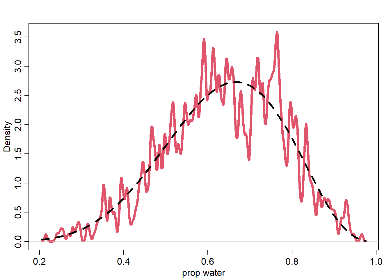
Analyze Sample + Summarize
<- rbeta (1e3 , 6 + 1 , 3 + 1 )dens (post_samples, lwd = 4 , col = 2 , xlab = "prop water" , adj = 0.1 )curve (dbeta (x, 6 + 1 , 3 + 1 ), add = T, lty = 2 , lwd = 3 )
posterior prediction = “what would we bet?”
how many W’s do we expect to see in the next 10 tosses
for each sample of post dist, we can create a predictive distribution, then posterior predictive
incorporates uncertainty from posterior distribution
<- rbeta (1e4 , 6 + 1 , 3 + 1 )<- sapply (post_samples, function (p) sum (sim_globe (p, 10 )== "W" ))<- table (pred_post)#for (i in 0:10) lines(c(i,i),c(0,tab_post[i+1]), lwd = 4, col = 4)
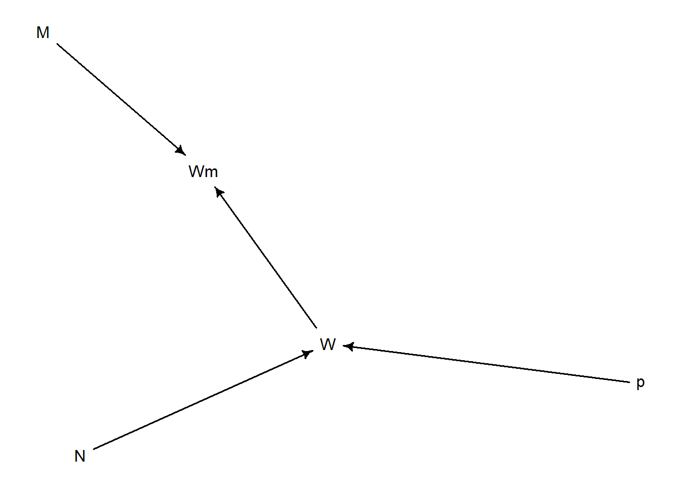
Misclassification (Bonus Round)
library (dagitty)library (rethinking)<- dagitty ("dag { p -> W N -> W W -> Wm M -> Wm }" )drawdag (d)
incorporate measurement error with x (error rate of 10%)
<- function (p = 0.7 , N = 9 , x = 0.1 ){<- sample (c ("W" , "L" ), size = N, prob = c (p, 1 - p), replace = T)<- ifelse (runif (N) < x,ifelse (true_sample == "W" , "L" , "W" ),return (obs_sample)