Homework - Week 05

Q1

The data in data(NWOGrants) are outcomes for scientific funding applications for the Netherlands Organization for Scientific Research (NWO) from 2010–2012 (see van der Lee and Ellemers doi:10.1073/pnas.1510159112). These data have a structure similar to the UCBAdmit data discussed in Chapter 11 and in lecture. There are applications and each has an associated gender (of the lead researcher). But instead of departments, there are disciplines. Draw a DAG for this sample. Then use the backdoor criterion and a binomial GLM to estimate the TOTAL causal effect of gender on grant awards.

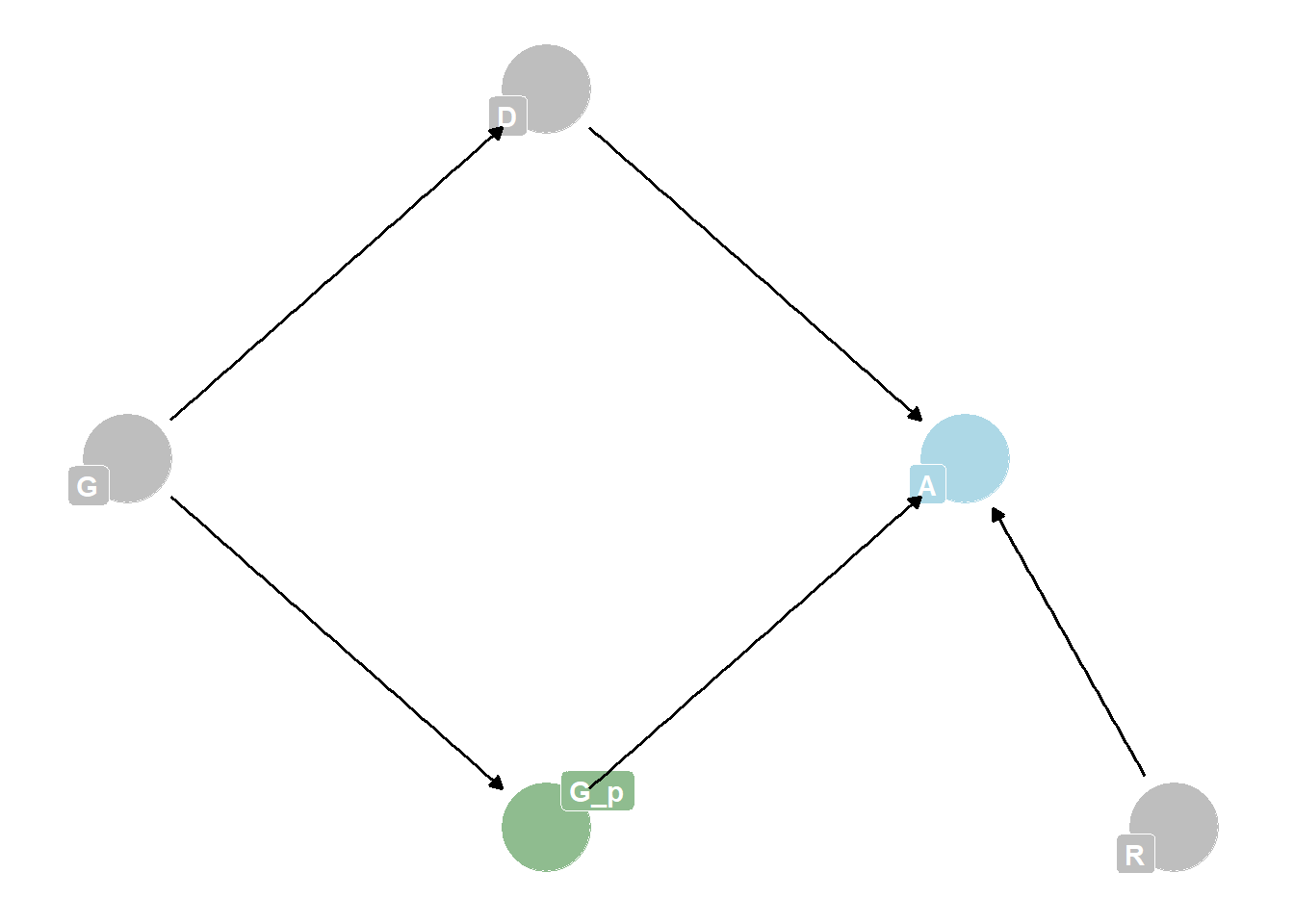
Total causal effect of gender requires no adjustment sets, although we could add referee ID to the model to help it fit better, as it is additional information in the system that is not connected through backdoor paths. I will model as:

$$ Awards_i | Applications_i Binomial(N_i, p_i) \ logit(p_i) = \ = [_f, _m] \ Normal(0, 1.5) \ Normal(0, 0.5)

$$ question: why do we use binomial and he uses Bernoulli?

mod1 <- tar_read(h05_q1_brms_sample)

# plot predicted draws for each group using modelled dataset
epred <- mod1 %>% 
  predicted_draws(newdata = NWOGrants)

ggplot(epred, aes(x = .prediction, fill = gender)) +
  stat_halfeye(alpha = 0.7) +
  labs(x = "Awards", y = "Density", fill = "Gender") +
  theme_classic() +
  theme(legend.position = "top")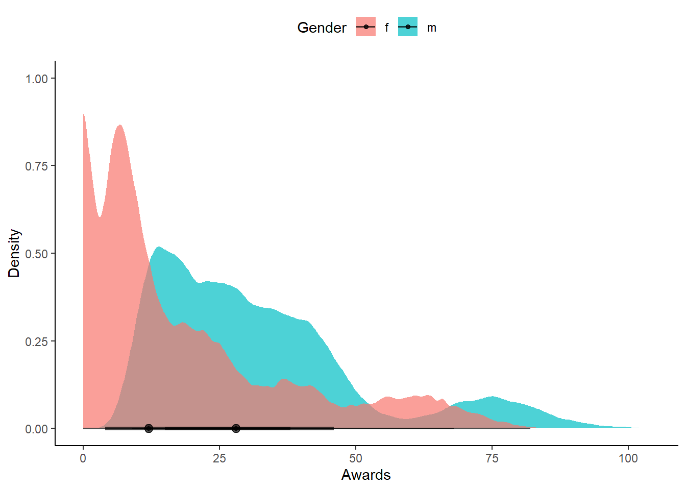

# calculate contrast using emmeans 
total_gender_effect <- mod1 %>% 
  emmeans(~ gender,
          # undo link transformation
          regrid = 'response') %>% 
  contrast(method = "pairwise") %>% 
  gather_emmeans_draws()

ggplot(total_gender_effect, aes(x = .value)) +
  stat_halfeye() +
  labs(x = "Total causal effect of gender (female - male)", y = "Density") +
  theme_classic() +
  theme(legend.position = "bottom")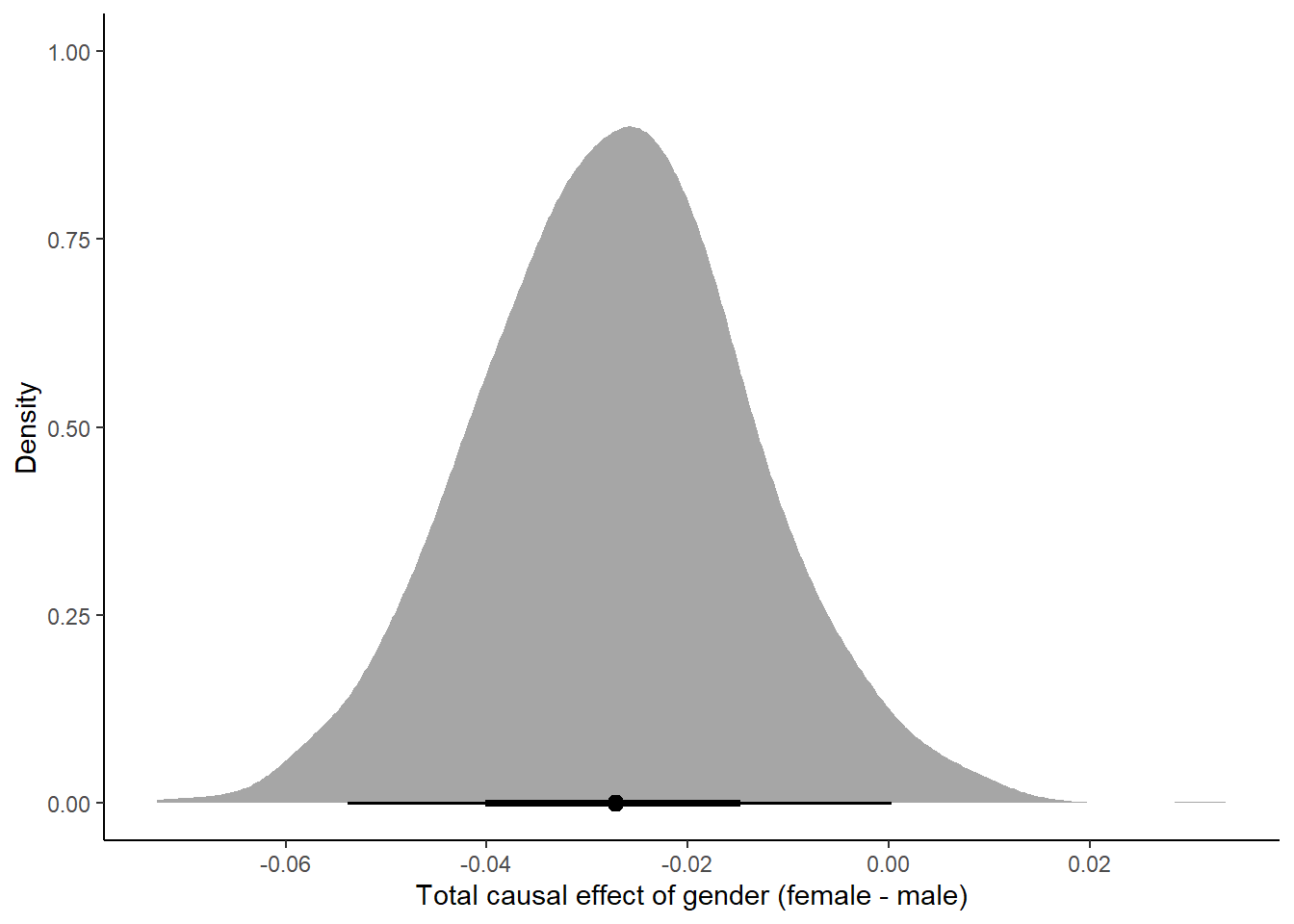

Q2

Now estimate the DIRECT causal effect of gender on grant awards. Use the same DAG as above to justify one or more binomial models. Compute the average direct causal effect of gender, weighting each discipline in proportion to the number of applications in the sample. Refer to the marginal effect example in Lecture 9 for help.

To calculate the direct causal effect of gender on grant awards, add discipline to the model.

$$ Awards_i | Applications_i Binomial(N_i, p_i) \ logit(p_i) = \ Normal(0, 1.5) \ Normal(0, 0.5)

$$

mod2 <- tar_read(h05_q2_brms_sample)

# calculate contrast using emmeans 
direct_gender_effect <- mod2 %>% 
  emmeans(~ gender|discipline,
          # undo link transformation
          regrid = 'response') %>% 
  contrast(method = "pairwise") %>% 
  gather_emmeans_draws()

ggplot(direct_gender_effect, aes(x = .value, fill = discipline)) +
  stat_halfeye(alpha = 0.5) +
  labs(x = "Direct causal effect of gender (female - male)", y = "Density", fill = "") +
  theme_classic() +
  theme(legend.position = "top")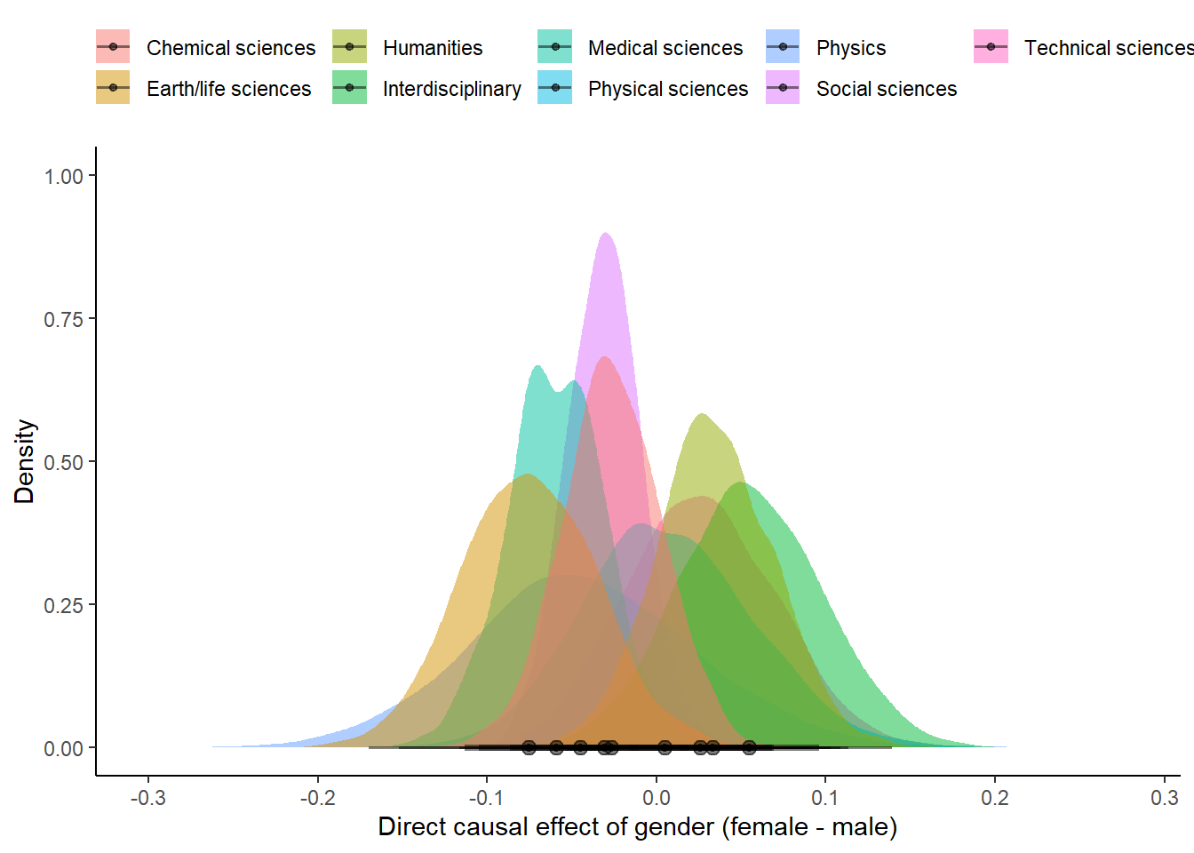

Weight the sample based on number of applications (post-stratification):

post <- NWOGrants %>%
  group_by(discipline) %>% 
  summarize(n_app = sum(applications)) %>% 
  ungroup() %>% 
  mutate(prop_app = n_app / sum(n_app)) %>% 
  right_join(., direct_gender_effect, by = "discipline") %>% 
  group_by(discipline, .draw) %>% 
  summarize(post_predict = sum(.value * prop_app)) %>% 
  mean_qi(post_predict)

ggplot(data = post, aes(x = post_predict, xmin = .lower, xmax = .upper, y = discipline)) + 
  geom_pointrange(color = "orange2", linewidth = 0.8, fatten = 2)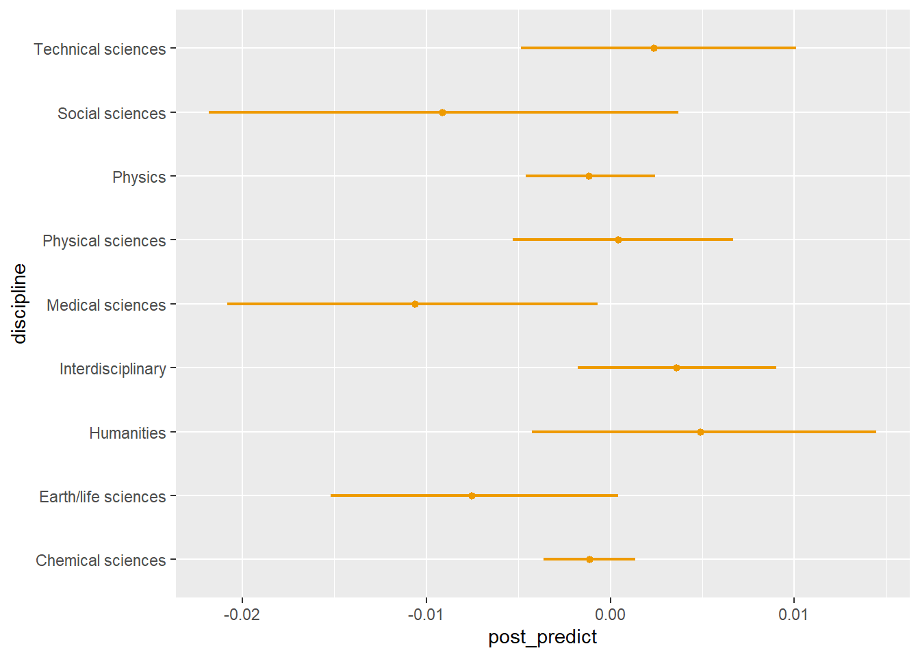

Q3 (optional)

The data in data(UFClefties) are the outcomes of 205 Ultimate Fighting Championship (UFC) matches (see ?UFClefties for details). It is widely believed that left-handed fighters (aka “Southpaws”) have an advantage against right-handed fighters, and left-handed men are indeed over-represented among fighters (and fencers and tennis players) compared to the general population. Estimate the average advantage, if any, that a left-handed fighter has against right-handed fighters. Based upon your estimate, why do you think left-handers are over-represented among UFC fighters?