Lecture 10 - Counts & Hidden Confounds
Rose / Thorn
Rose: qualitative data!!
Thorn:
Generalized Linear Models
Expected value is some function (link function) of an additive combination of parameters
interpretation that changes, not computation - no longer simply an additive combination of parameters
- uniform changes in predictor not uniform changes in prediction
all predictor variables interact and moderate one another
inlfuences predictions and uncertainty of predictions
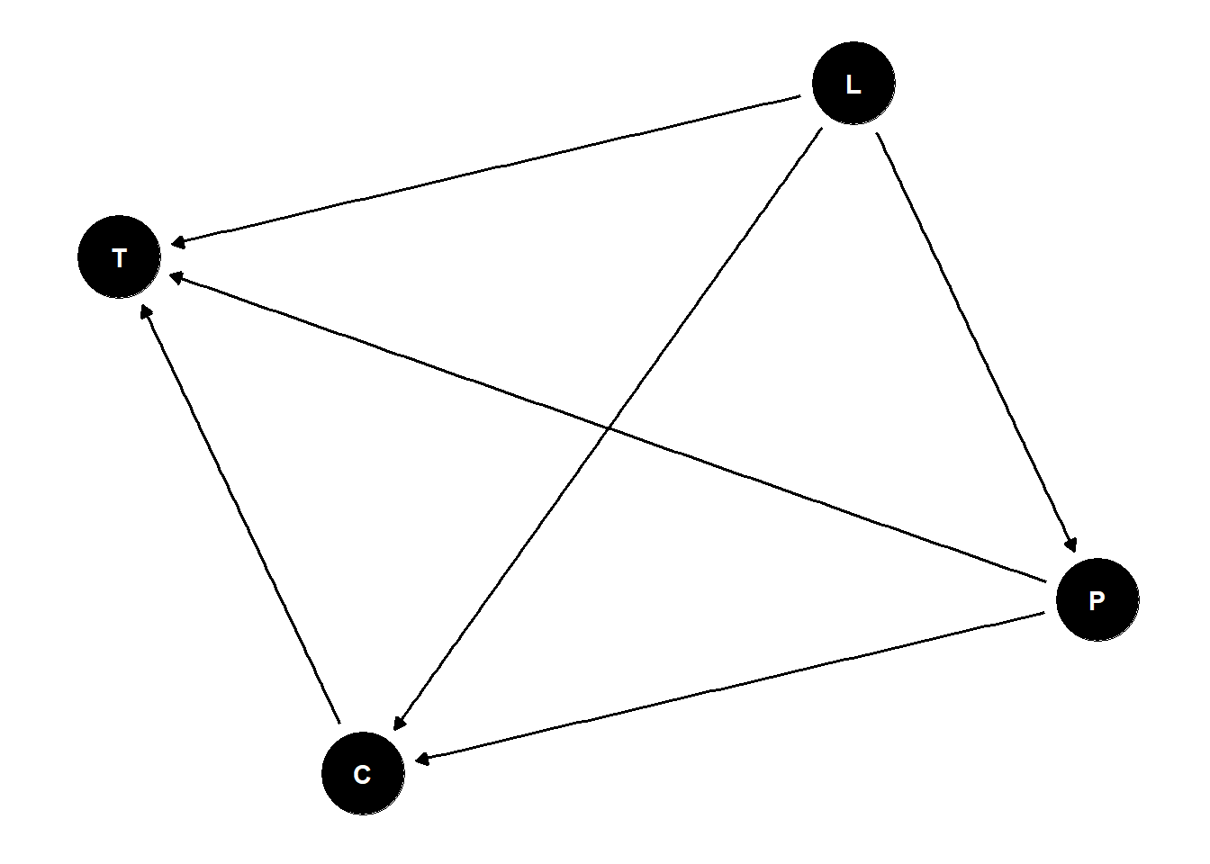
Confounded Admissions
ability is the most easy to imagine confound for admissions
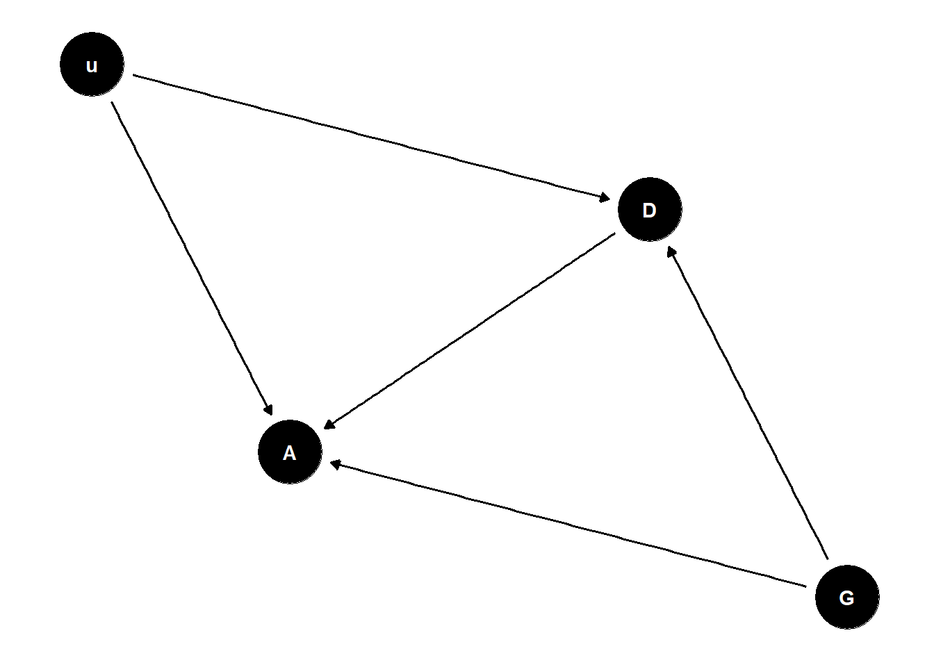
include confound in the model (u):
- Bernoulli variable 0, 1 - 1 is extremely high achieving individuals that are 10% of the population, everyone else is average
gender 1 individuals anticipate gender discrimination in department 2, so if they are average they will avoid it but if they are exceptional they will still apply
# continuing from UCBadmit example
# what happens when there is a confound?

set.seed(17)
N <- 2000 # number of applicants
# even gender distribution
G <- sample( 1:2 , size=N , replace=TRUE )
# sample ability, high (1) to average (0)
# unobserved common cause
u <- rbern(N,0.1)
# gender 1 tends to apply to department 1, 2 to 2
# and G=1 with greater ability tend to apply to 2 as well
D <- rbern( N , ifelse( G==1 , u*0.5 , 0.8 ) ) + 1
# matrix of acceptance rates [dept,gender]
accept_rate_u0 <- matrix( c(0.1,0.1,0.1,0.3) , nrow=2 )
accept_rate_u1 <- matrix( c(0.2,0.3,0.2,0.5) , nrow=2 )
# simulate acceptance
p <- sapply( 1:N , function(i)
    ifelse( u[i]==0 , accept_rate_u0[D[i],G[i]] , accept_rate_u1[D[i],G[i]] ) )
A <- rbern( N , p )

table(G,D)
table(G,A)

dat_sim <- list( A=A , D=D , G=G )

# total effect gender
m1 <- ulam(
    alist(
        A ~ bernoulli(p),
        logit(p) <- a[G],
        a[G] ~ normal(0,1)
    ), data=dat_sim , chains=4 , cores=4 )

post1 <- extract.samples(m1)
post1$fm_contrast <- post1$a[,1] - post1$a[,2]
precis(post1)

# direct effects - now confounded!
m2 <- ulam(
    alist(
        A ~ bernoulli(p),
        logit(p) <- a[G,D],
        matrix[G,D]:a ~ normal(0,1)
    ), data=dat_sim , chains=4 , cores=4 )

precis(m2,3)- second model stratifies through department is now confounded because we’ve added a common cause, ability
# contrast
post2 <- extract.samples(m2)
post2$fm_contrast_D1 <- post2$a[,1,1] - post2$a[,2,1]
post2$fm_contrast_D2 <- post2$a[,1,2] - post2$a[,2,2]
precis(post2)

dens( post2$fm_contrast_D1 , lwd=4 , col=4 , xlab="F-M contrast in each department" )
dens( post2$fm_contrast_D2 , lwd=4 , col=2 , add=TRUE )
abline(v=0,lty=3)

dens( post2$a[,1,1] , lwd=4 , col=2 , xlim=c(-3,1) )
dens( post2$a[,2,1] , lwd=4 , col=4 , add=TRUE )
dens( post2$fm_contrast_D1 , lwd=4 , add=TRUE )

dens( post2$a[,1,2] , lwd=4 , col=2 , add=TRUE , lty=4 )
dens( post2$a[,2,2] , lwd=4 , col=4 , add=TRUE , lty=4)
dens( post2$fm_contrast_D2 , lwd=4 , add=TRUE , lty=4)
probability distribution of probabilities because we’re modelling probability
confound happens because exceptional individuals don’t apply to department 1, they apply to department 2 and so it looks like department 1 is discriminating when its not because its getting lower quality applicants
- department 2 appears to have no discrimination but it does have it, for the opposite reason. they are only admitting higher ability applicants of a certain gender
masking effect - sorting can mask a lot of things
Collider Bias
We can estimate total causal effect of G but it isn’t what we want (not useful for policy)
We cannot estimate direct effect of department or gender
Citation vs Membership
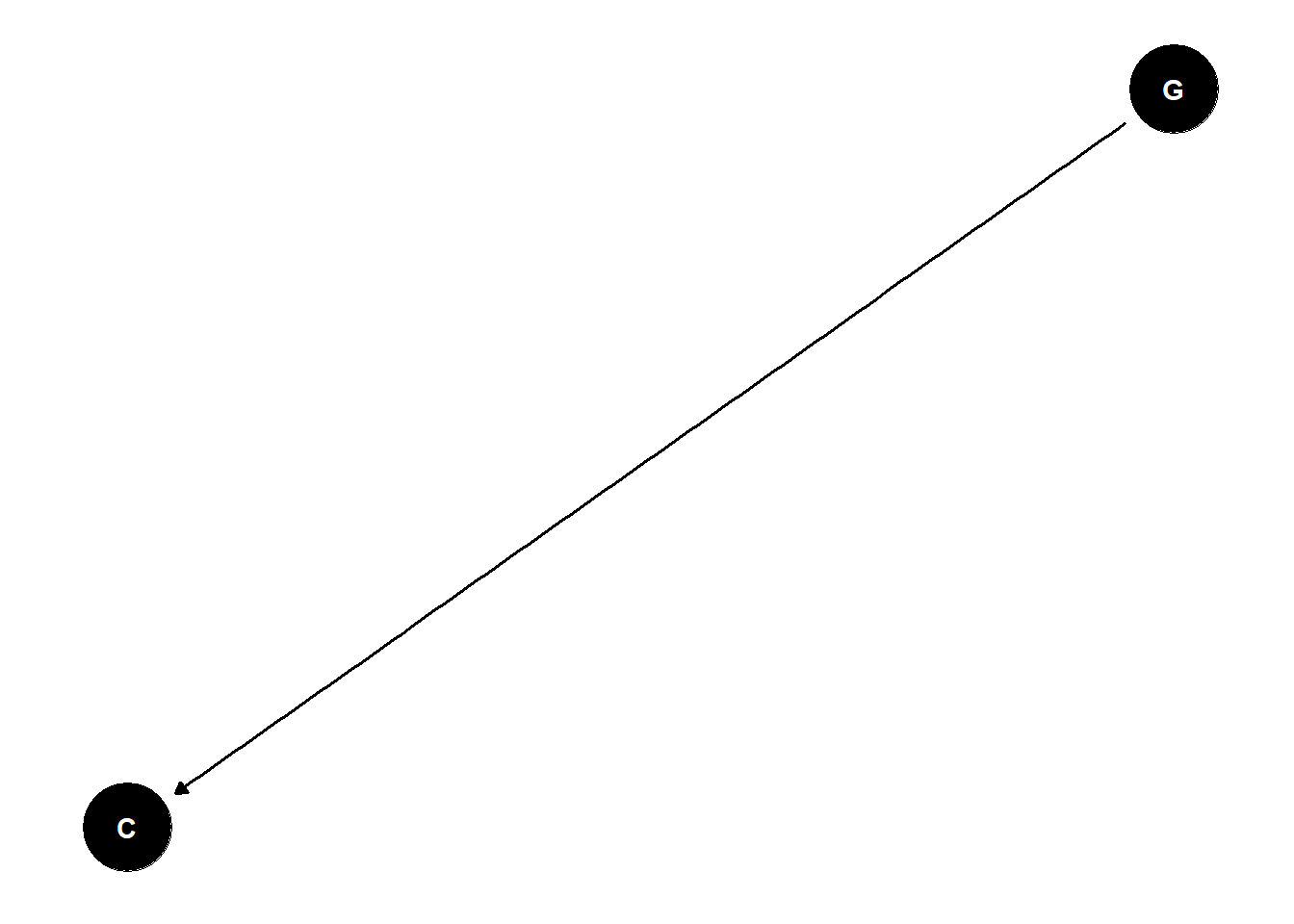
paper one concludes that gender results in lower citation rates for women
paper two concludes that women get elected more controlling for citations
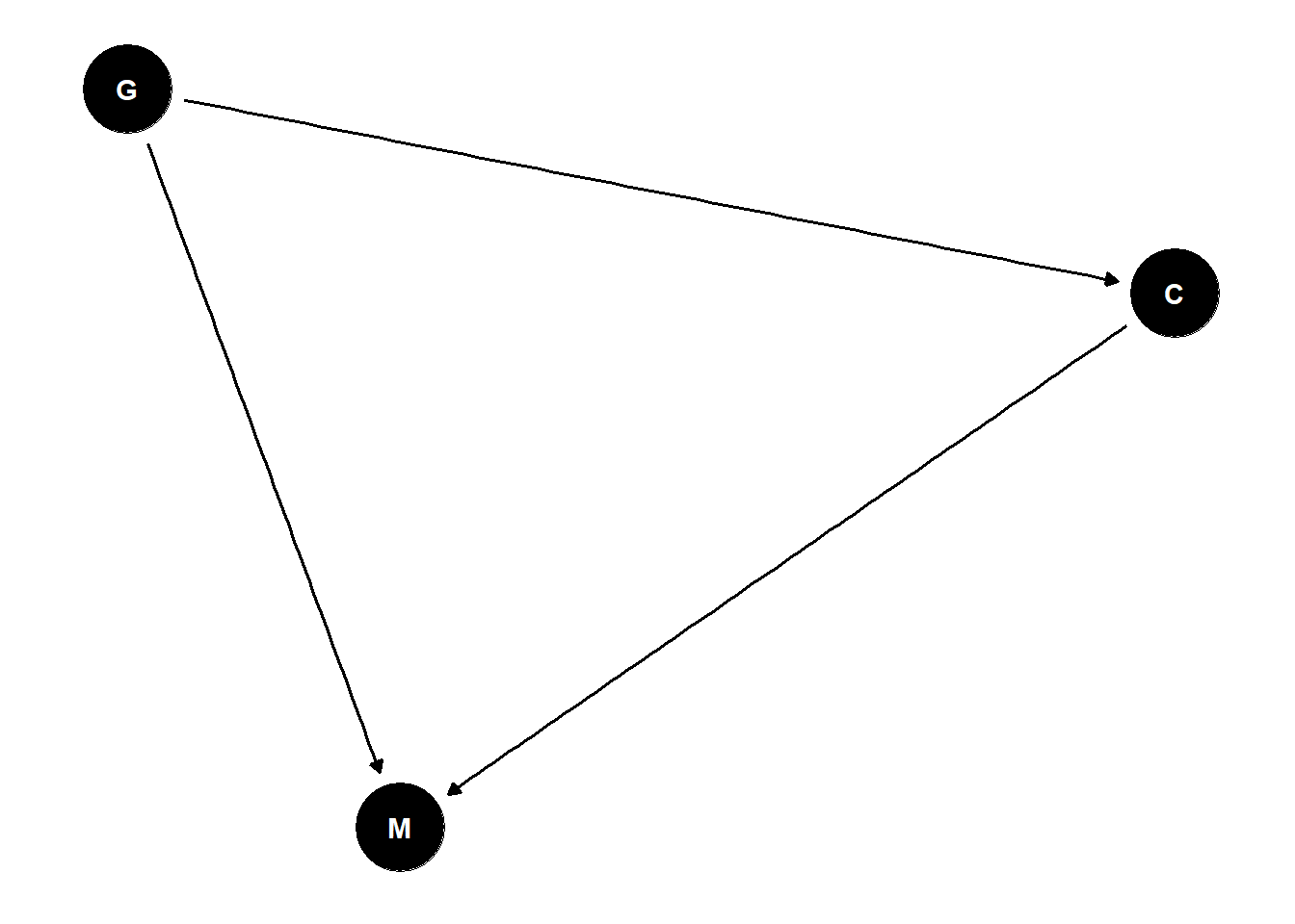
Citation Networks
very plausible that there is quality differences among members of the academy but they are often hidden
citations is a post-treatment variable (and stratifying by post-treatment variable is dangerous because it can activate collider bias)
- if women are less likely to get citations because of discrimination, it is probably that women elected to the NAS with less citations have a higher quality
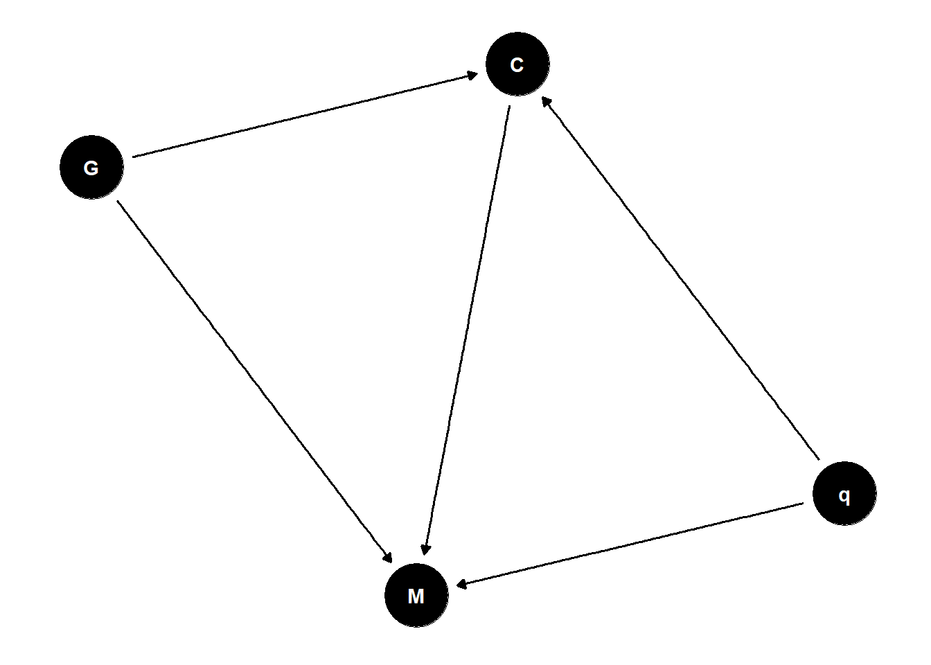
in the absence of strong causal assumptions, we can’t conclude anything
proxies for quality are often poor proxies (e.g., citations)
if you want causal inference, you must make causal assumptions
Sensitivity Analysis
what are the implications of what we don’t know?
assume confound exists, model its consequences for different strengths/kinds of influence
how strong must the confound be to change conclusions?
include quality as an unobserved variable
- change parameter size/strength to test the effect of unobserved confound
\[ A_i \sim Bernoulli(p_i) \\ logit(p_i) = \alpha[G_i, D_i] +\beta_{G[i]}u_i \]
- first model models total effect of gender on admissions with an unknown confound (quality)
\[ (D_i = 2) \sim Bernoulli(q_i) \\ logit(q_i) = \delta[G_i] + \gamma_{G[i]}u_i \]
- second model investigates the effect of how people apply to departments
\(u_j \sim Normal(0, 1)\)
\(u_i\) = ability
# sensitivity

dat_sim$D2 <- ifelse( D==2 , 1 , 0 )
dat_sim$b <- c(1,1)
dat_sim$g <- c(1,0)
dat_sim$N <- length(dat_sim$D2)

m3s <- ulam(
    alist(
        # A model
        A ~ bernoulli(p),
        logit(p) <- a[G,D] + b[G]*u[i],
        matrix[G,D]:a ~ normal(0,1),

        # D model
        D2 ~ bernoulli(q),
        logit(q) <- delta[G] + g[G]*u[i],
        delta[G] ~ normal(0,1),

        # declare unobserved u
        vector[N]:u ~ normal(0,1)
    ), data=dat_sim , chains=4 , cores=4 )

precis(m3s,3,pars=c("a","delta"))

post3s <- extract.samples(m3s)
post3s$fm_contrast_D1 <- post3s$a[,1,1] - post3s$a[,2,1]
post3s$fm_contrast_D2 <- post3s$a[,1,2] - post3s$a[,2,2]

dens( post2$fm_contrast_D1 , lwd=1 , col=4 , xlab="F-M contrast in each department" , xlim=c(-2,1) )
dens( post2$fm_contrast_D2 , lwd=1 , col=2 , add=TRUE )
abline(v=0,lty=3)
dens( post3s$fm_contrast_D1 , lwd=4 , col=4 , add=TRUE )
dens( post3s$fm_contrast_D2 , lwd=4 , col=2 , add=TRUE )

plot( jitter(u) , apply(post3s$u,2,mean) , col=ifelse(G==1,2,4) , lwd=3 )
you can say the strength of the confound needed to undo the results you found
important thing to report - don’t pretend confounds don’t exist
can’t eliminate possibility of confounding
a lot of the most important science cannot be done experimentally so we need to be able to do these things
Poisson Counts
total count is not binomial: no maximum
- Poisson distribution: very high maximum and very low probability of each success
Poisson distribution uses the log link - must be positive
exponential scaling can be surprising
large priors makes extremely long tails with very large values
want higher mean, lower variance
\[ Y_i \sim Poisson(\lambda_i) \\ log(\lambda_i) = \alpha + \beta x_i \\ \lambda_i = exp(\alpha + \beta x_i) \]
To add contact as an interaction term where C is contact:
- \[ Y_i \sim Poisson(\lambda_i) \\ log(\lambda_i) = \alpha_{C[i]} + \beta_{C[i]} log(P_i) \\ \alpha_j \sim Normal(3, 0.5) \\ \beta_j \sim Normal(0, 0.2) \]
# model

library(rethinking)
data(Kline)
d <- Kline
d$P <- scale( log(d$population) )
d$contact_id <- ifelse( d$contact=="high" , 2 , 1 )

dat <- list(
    T = d$total_tools ,
    P = d$P ,
    C = d$contact_id )

# intercept only
m11.9 <- ulam(
    alist(
        T ~ dpois( lambda ),
        log(lambda) <- a,
        a ~ dnorm( 3 , 0.5 )
    ), data=dat , chains=4 , log_lik=TRUE )

# interaction model
m11.10 <- ulam(
    alist(
        T ~ dpois( lambda ),
        log(lambda) <- a[C] + b[C]*P,
        a[C] ~ dnorm( 3 , 0.5 ),
        b[C] ~ dnorm( 0 , 0.2 )
    ), data=dat , chains=4 , log_lik=TRUE )

compare( m11.9 , m11.10 , func=PSIS )

k <- PSIS( m11.10 , pointwise=TRUE )$k
plot( dat$P , dat$T , xlab="log population (std)" , ylab="total tools" ,
    col=ifelse( dat$C==1 , 4 , 2 ) , lwd=4+4*normalize(k) ,
    ylim=c(0,75) , cex=1+normalize(k) )
# set up the horizontal axis values to compute predictions at
P_seq <- seq( from=-1.4 , to=3 , len=100 )

# predictions for C=1 (low contact)
lambda <- link( m11.10 , data=data.frame( P=P_seq , C=1 ) )
lmu <- apply( lambda , 2 , mean )
lci <- apply( lambda , 2 , PI )
lines( P_seq , lmu , lty=2 , lwd=1.5 )
shade( lci , P_seq , xpd=TRUE , col=col.alpha(4,0.3) )

# predictions for C=2 (high contact)
lambda <- link( m11.10 , data=data.frame( P=P_seq , C=2 ) )
lmu <- apply( lambda , 2 , mean )
lci <- apply( lambda , 2 , PI )
lines( P_seq , lmu , lty=1 , lwd=1.5 )
shade( lci , P_seq , xpd=TRUE , col=col.alpha(2,0.3))

identify( dat$P , dat$T , d$culture )

# natural scale now

plot( d$population , d$total_tools , xlab="population" , ylab="total tools" ,
    col=ifelse( dat$C==1 , 4 , 2 ) , lwd=4+4*normalize(k) ,
    ylim=c(0,75) , cex=1+normalize(k) )
P_seq <- seq( from=-5 , to=3 , length.out=100 )
# 1.53 is sd of log(population)
# 9 is mean of log(population)
pop_seq <- exp( P_seq*1.53 + 9 )
lambda <- link( m11.10 , data=data.frame( P=P_seq , C=1 ) )
lmu <- apply( lambda , 2 , mean )
lci <- apply( lambda , 2 , PI )
lines( pop_seq , lmu , lty=2 , lwd=1.5 )
shade( lci , pop_seq , xpd=TRUE , col=col.alpha(4,0.3))

lambda <- link( m11.10 , data=data.frame( P=P_seq , C=2 ) )
lmu <- apply( lambda , 2 , mean )
lci <- apply( lambda , 2 , PI )
lines( pop_seq , lmu , lty=1 , lwd=1.5 )
shade( lci , pop_seq , xpd=TRUE , col=col.alpha(2,0.3) )

identify( d$population , d$total_tools , d$culture )
number of effective parameters penalty shows how well the model performs after you drop individual data points
- therefore models with more parameters often have lower effective parameters
gamma-Poisson is the appropriate analog to a student t-test - wider tails and more robust
improve scientific model
people produce innovations so population and contact both innovate but there is also loss
\[ \Delta T = \alpha_C P^{\beta_C} - \gamma T \]
\(\Delta T\) = change in tools
\(\alpha\) = innovation rate
\(\beta\) = diminishing returns
\(\gamma\) = loss
T = number of tools
C = contact
set equation to 0 and solve for T then insert into your model
\[ \hat{T} = \frac {\alpha_C P^{\beta_C}} {\gamma} \\ T_i \sim Poisson (\lambda_i) \\ \lambda_i = \hat{T} \]
must constrain all parameters to be positive
# innovation/loss model

dat2 <- list( T=d$total_tools, P=d$population, C=d$contact_id )
m11.11 <- ulam(
    alist(
        T ~ dpois( lambda ),
        lambda <- exp(a[C])*P^b[C]/g,
        a[C] ~ dnorm(1,1),
        b[C] ~ dexp(1),
        g ~ dexp(1)
    ), data=dat2 , chains=4 , cores=4 , log_lik=TRUE )

precis(m11.11,2)

plot( d$population , d$total_tools , xlab="population" , ylab="total tools" ,
    col=ifelse( dat$C==1 , 4 , 2 ) , lwd=4+4*normalize(k) ,
    ylim=c(0,75) , cex=1+normalize(k) )
P_seq <- seq( from=-5 , to=3 , length.out=100 )- still need to deal with location as confound
Count GLMs
distributions from constraints
maximum entropy priors: binomial, Poisson, and extensions
robust regressions: beta-binomial, gamma-Poisson
Simpson’s Paradox
reversal of an association when groups are combined or separated within the dataset
the reversal is purely statistical - no way to understand it without causal assumptions
non-linear haunting
there’s a positive effect in both groups but it cannot be estimated from this sample
just because your distribution overlaps zero, doesn’t mean the effect is null