Homework - Week 06
Q1
Conduct a prior predictive simulation for the Reedfrog model. By this I mean to simulate the prior distribution of tank survival probabilities αj. Start by using this prior:
$$
_j Normal({}, )
\[ \] {} Normal(0, 1)
$$
$$ Exponential(1)
$$
Be sure to transform the αj values to the probability scale for plotting and summary. How does increasing the width of the prior on σ change the prior distribution of αj? You might try Exponential(10) and Exponential(0.1) for example.
r <- reedfrogs %>%
  mutate(tank = 1:nrow(reedfrogs))

exp1 <- tar_read(h06_q1_a)
exp10 <- tar_read(h06_q1_b)
exp0.1 <- tar_read(h06_q1_c)

# Prior Predictive Simulation 1
exp1 %>%
  add_predicted_draws(newdata = r,
                  re_formula = NA) %>%
  ggplot() +
  stat_pointinterval(aes(tank, .prediction/density), .width = 0.95) +
  geom_point(aes(x = tank, y = surv/density), colour = 'red') +
  geom_hline(yintercept = 0.8, linetype = 2, linewidth = 1/4) +
  geom_vline(xintercept = c(16.5, 32.5), linewidth = 1/4, color = "grey25") +
  labs(y = 'Prior predicted survival rate', x = 'Tank') +
  ggtitle("sigma = 1") +
  theme_classic()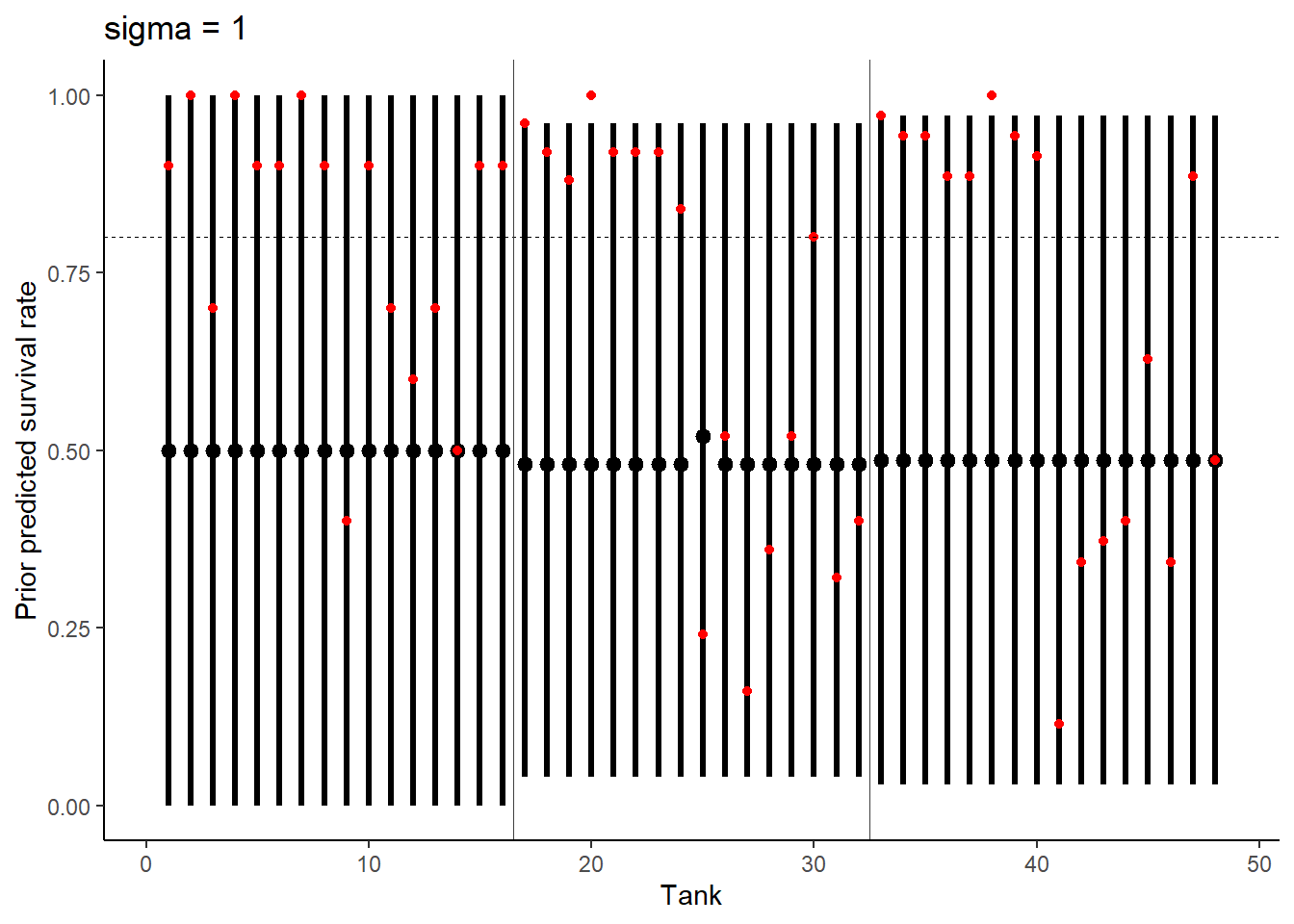
# Prior Predictive Simulation 2
exp10 %>%
  predicted_draws(newdata = r,
                  re_formula = NA) %>%
  ggplot() +
  stat_pointinterval(aes(tank, .prediction/density), .width = 0.95) +
  geom_point(aes(x = tank, y = surv/density), colour = 'red') +
  geom_hline(yintercept = 0.8, linetype = 2, linewidth = 1/4) +
  geom_vline(xintercept = c(16.5, 32.5), linewidth = 1/4, color = "grey25") +
  labs(y = 'Prior predicted survival rate', x = 'Tank') +
  ggtitle("sigma = 10") +
  theme_classic()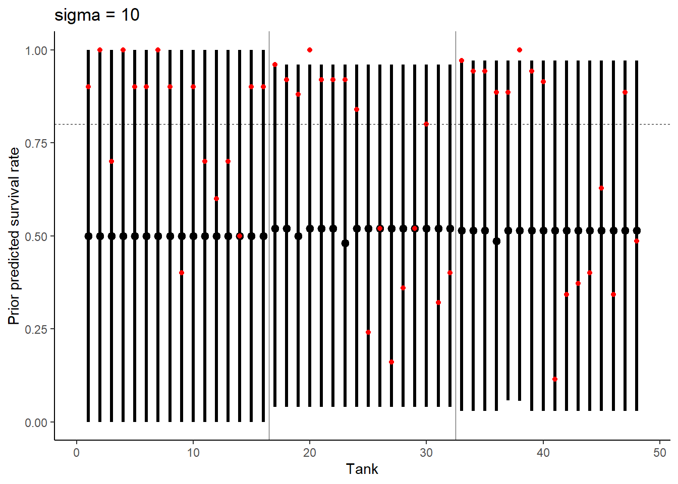
# Prior Predictive Simulation 3
exp0.1 %>%
  predicted_draws(newdata = r,
                  re_formula = NA) %>%
  ggplot() +
  stat_pointinterval(aes(tank, .prediction/density), .width = 0.95) +
  geom_point(aes(x = tank, y = surv/density), colour = 'red') +
  geom_hline(yintercept = 0.8, linetype = 2, linewidth = 1/4) +
  geom_vline(xintercept = c(16.5, 32.5), linewidth = 1/4, color = "grey25") +
  labs(y = 'Prior predicted survival rate', x = 'Tank') +
  ggtitle("sigma = 0.1") +
  theme_classic()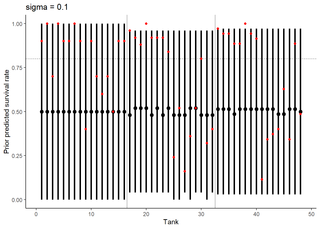
NOTE: did this wrong!! This is not \(\alpha_j\), this is \(\bar{\alpha}\) . Checked Richard’s answers and I should be visualizing the pooled individual effects - going to attempt this here:
exp1 %>%
  add_predicted_draws(newdata = r,
                  re_formula = NA) %>%
  ggplot() +
  stat_histinterval(aes(x = .prediction/density)) +
  labs(x = "Prior predicted survival", y = "Density") +
  ggtitle(label = "Sigma = 1") +
  theme_classic()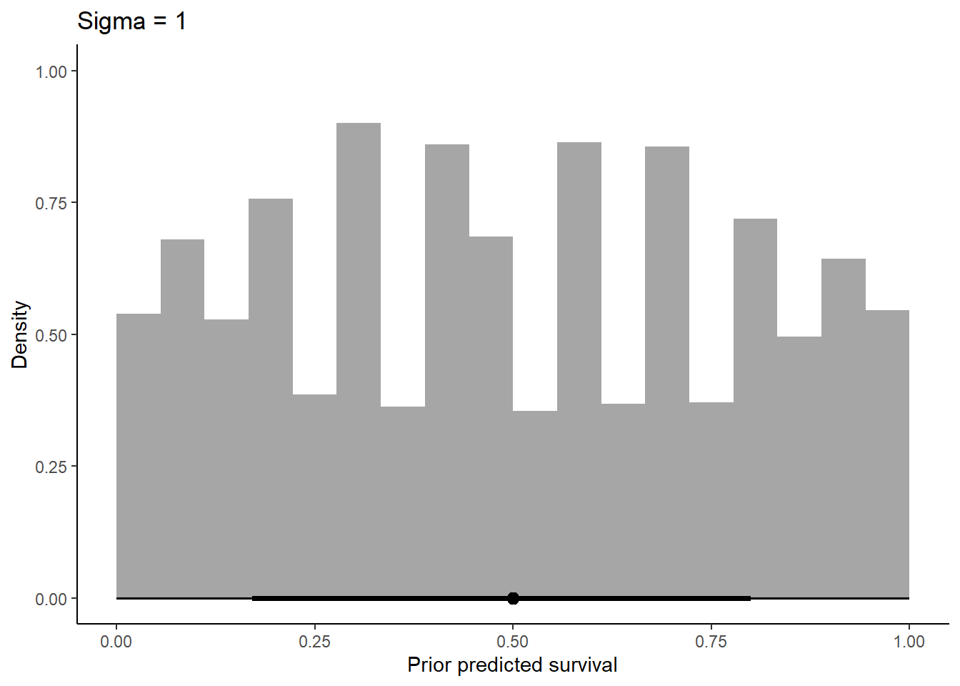
exp10 %>%
  add_predicted_draws(newdata = r) %>%
  ggplot() +
  stat_histinterval(aes(x = .prediction/density)) +
  labs(x = "Prior predicted survival", y = "Density") +
  ggtitle(label = "Sigma = 10") +
  theme_classic()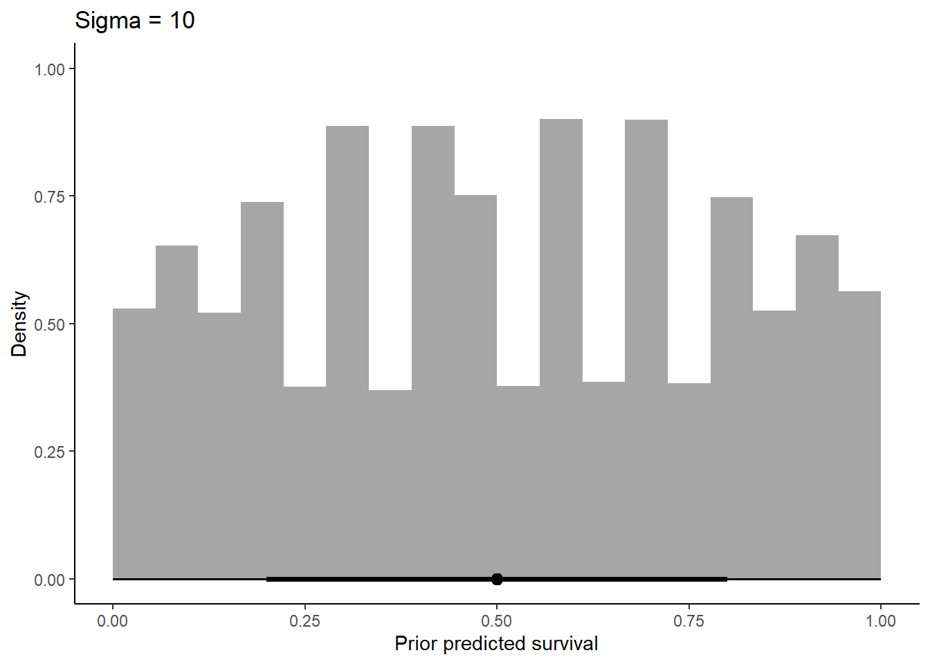
exp0.1 %>%
  add_predicted_draws(newdata = r) %>%
  ggplot() +
  stat_histinterval(aes(x = .prediction/density)) +
  labs(x = "Prior predicted survival", y = "Density") +
  ggtitle(label = "Sigma = 0.1") +
  theme_classic()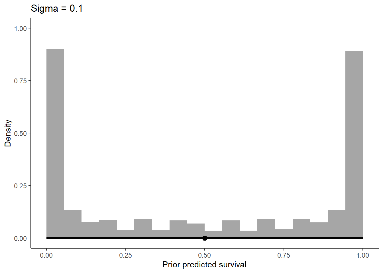
Increasing sigma evens out the probability distribution instead of having it bunched in two extremes like we see at 0.1
Here I am looking at response instead of the parameters - to plot the parameter distribution I can use mcmc_areas.
Q2
Revisit the Reedfrog survival data,
data(reedfrogs). Start with the varying effects model from the book and lecture. Then modify it to estimate the causal effects of the treatment variables pred and size, including how size might modify the effect of predation. An easy approach is to estimate an effect for each combination of pred and size. Justify your model with a DAG of this experiment.
The DAG presented in the lecture appears as:
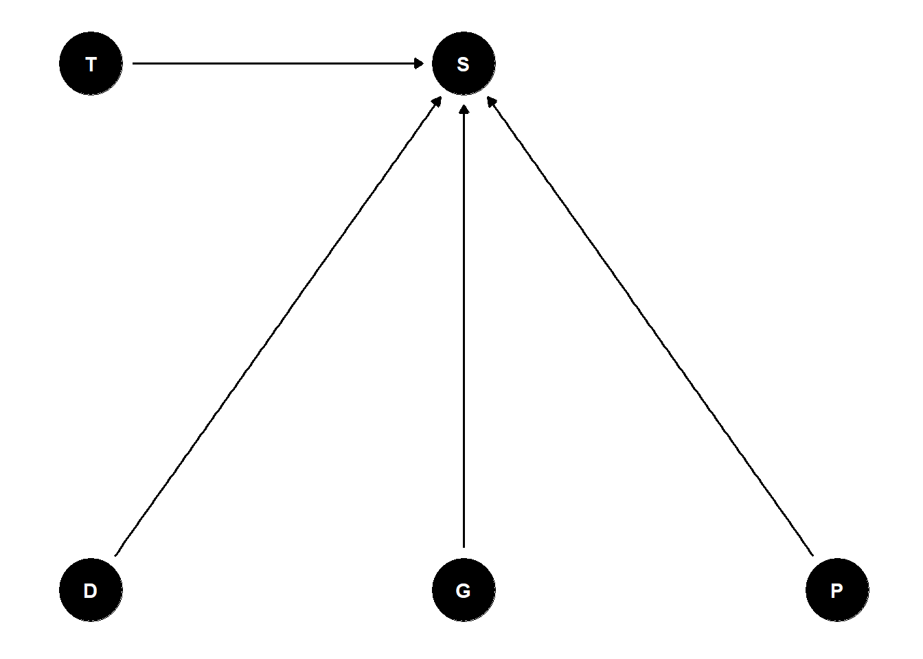
I mostly agree with this, although I think that in a natural setting the DAG would look different and there would be confounds. In this case, we can add everything to the model and independently examine the effects (total and direct are the same) of each variable. However, in Richard’s answers he has an interaction between predation (P) and size (G) - which makes sense. Larger individuals are more likely to be noticed and predated upon.
So my model looks like:
m <- tar_read(h06_q2_brms_sample)

print(m$formula)
surv | trials(density) ~ 1 + pred * size + (1 | tank) prior_summary(m) prior class coef group resp dpar nlpar lb ub
normal(0, 1) b
normal(0, 1) b predpred
normal(0, 1) b predpred:sizesmall
normal(0, 1) b sizesmall
normal(0, 1.5) Intercept
exponential(0.1) sd 0
exponential(0.1) sd tank 0
exponential(0.1) sd Intercept tank 0
source
user
(vectorized)
(vectorized)
(vectorized)
user
user
(vectorized)
(vectorized)summary(m) Family: binomial
Links: mu = logit
Formula: surv | trials(density) ~ 1 + pred * size + (1 | tank)
Data: h06_q2_brms_data (Number of observations: 48)
Draws: 4 chains, each with iter = 2000; warmup = 1000; thin = 1;
total post-warmup draws = 4000
Group-Level Effects:
~tank (Number of levels: 48)
Estimate Est.Error l-95% CI u-95% CI Rhat Bulk_ESS Tail_ESS
sd(Intercept) 0.78 0.15 0.52 1.12 1.00 1651 2249
Population-Level Effects:
Estimate Est.Error l-95% CI u-95% CI Rhat Bulk_ESS Tail_ESS
Intercept 2.44 0.30 1.86 3.02 1.00 1979 2776
predpred -2.67 0.38 -3.38 -1.89 1.00 1370 1974
sizesmall 0.20 0.39 -0.56 0.94 1.00 2160 2645
predpred:sizesmall 0.47 0.49 -0.50 1.43 1.00 1609 2093
Draws were sampled using sample(hmc). For each parameter, Bulk_ESS
and Tail_ESS are effective sample size measures, and Rhat is the potential
scale reduction factor on split chains (at convergence, Rhat = 1).brms eats the comparative levels, so we need to push them out (and make figures anyways!)
m %>%
  add_epred_draws(newdata = r,
                  re_formula = NA) %>%
  rowwise() %>%
  mutate(interaction = paste0(pred,"+", size)) %>%
  ggplot() +
  stat_halfeye(aes(y = interaction, x = .epred/density,)) +
  theme_classic() +
  labs(y = "", x = "Survival Rate")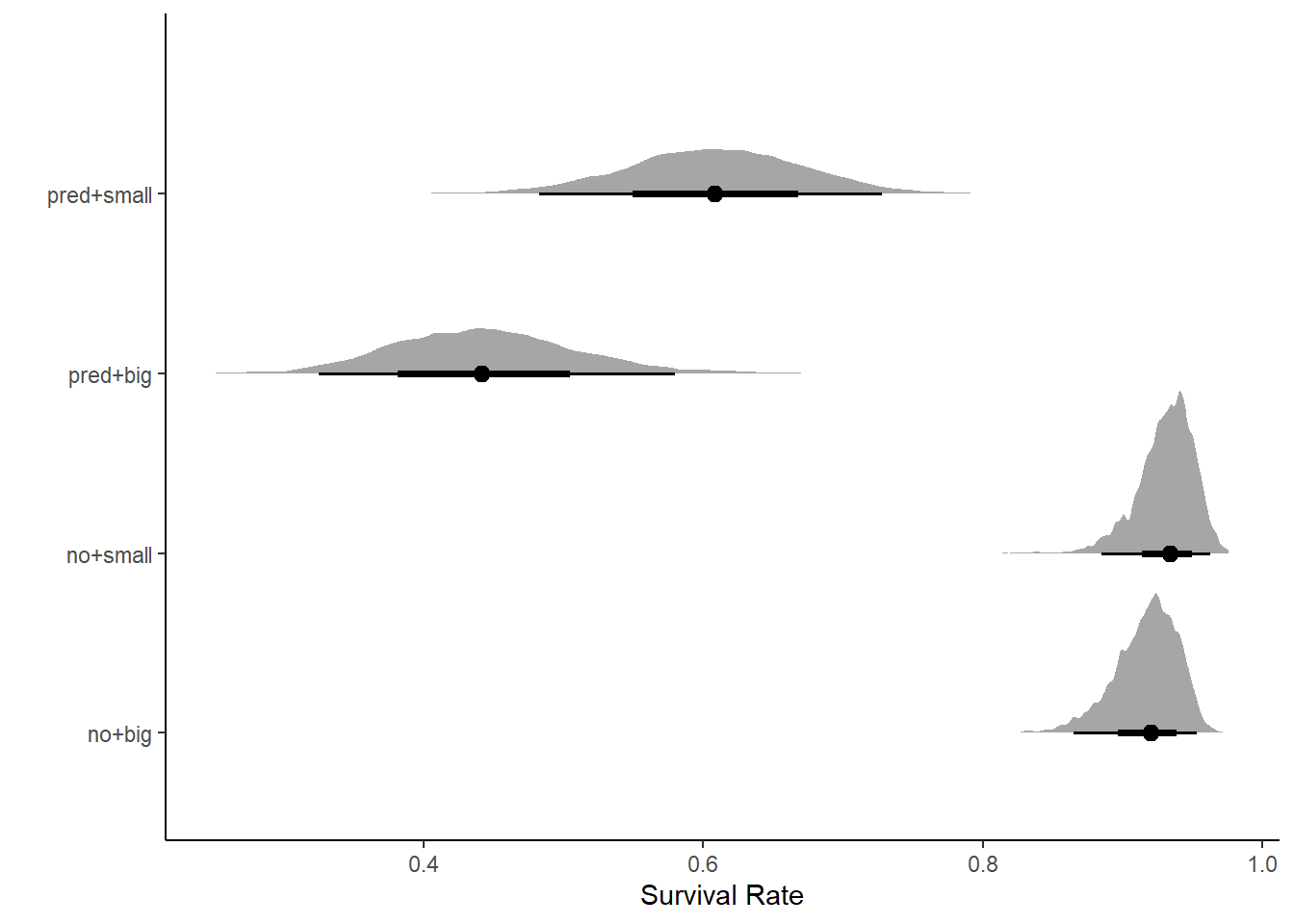
We see that size doesn’t matter in the absence of predators. Predators predictably decrease survival rate, but decrease survival rate for big tadpoles the most.
Ineractions are not in DAGs (always???)
Can also use emmeans here to do an easier visualization since the interaction is in the models
Q3 (optional)
Return to the Trolley data, data(Trolley), from Chapter 12. Define and fit a varying intercepts model for these data. By this I mean to add an intercept parameter for the individual participants to the linear model. Cluster the varying intercepts on individual participants, as indicated by the unique values in the id variable. Include action, intention, and contact as treatment effects of interest. Compare the varying intercepts model and a model that ignores individuals. What is the impact of individual variation in these data?
data(Trolley)


trolley <- Trolley %>%
  mutate(contact = as.factor(contact),
         action = as.factor(action),
         intention = as.factor(intention))

mod_naive <- tar_read(h06_q3b)
mod_ind <- tar_read(h06_q3)


summary(mod_naive)
Family: cumulative
Links: mu = logit; disc = identity
Formula: response ~ 1 + action + contact + intention
Data: trolley (Number of observations: 9930)
Draws: 4 chains, each with iter = 2000; warmup = 1000; thin = 1;
total post-warmup draws = 4000
Population-Level Effects:
Estimate Est.Error l-95% CI u-95% CI Rhat Bulk_ESS Tail_ESS
Intercept[1] -2.83 0.05 -2.93 -2.74 1.00 2463 2494
Intercept[2] -2.15 0.04 -2.24 -2.07 1.00 2808 2806
Intercept[3] -1.57 0.04 -1.65 -1.49 1.00 2903 3179
Intercept[4] -0.55 0.04 -0.62 -0.48 1.00 3079 3048
Intercept[5] 0.12 0.04 0.05 0.19 1.00 3421 3249
Intercept[6] 1.03 0.04 0.95 1.10 1.00 3774 3291
action1 -0.71 0.04 -0.79 -0.63 1.00 3393 3035
contact1 -0.96 0.05 -1.06 -0.86 1.00 3752 3051
intention1 -0.72 0.04 -0.79 -0.65 1.00 4429 2916
Family Specific Parameters:
Estimate Est.Error l-95% CI u-95% CI Rhat Bulk_ESS Tail_ESS
disc 1.00 0.00 1.00 1.00 NA NA NA
Draws were sampled using sampling(NUTS). For each parameter, Bulk_ESS
and Tail_ESS are effective sample size measures, and Rhat is the potential
scale reduction factor on split chains (at convergence, Rhat = 1).summary(mod_ind) Family: cumulative
Links: mu = logit; disc = identity
Formula: response ~ 1 + action + contact + intention + (1 | id)
Data: trolley (Number of observations: 9930)
Draws: 4 chains, each with iter = 2000; warmup = 1000; thin = 1;
total post-warmup draws = 4000
Group-Level Effects:
~id (Number of levels: 331)
Estimate Est.Error l-95% CI u-95% CI Rhat Bulk_ESS Tail_ESS
sd(Intercept) 1.88 0.08 1.73 2.06 1.01 627 1000
Population-Level Effects:
Estimate Est.Error l-95% CI u-95% CI Rhat Bulk_ESS Tail_ESS
Intercept[1] -3.98 0.12 -4.22 -3.76 1.01 414 816
Intercept[2] -3.06 0.11 -3.29 -2.85 1.01 382 895
Intercept[3] -2.28 0.11 -2.51 -2.07 1.01 369 860
Intercept[4] -0.81 0.11 -1.03 -0.60 1.01 347 726
Intercept[5] 0.23 0.11 0.01 0.44 1.01 336 765
Intercept[6] 1.63 0.11 1.41 1.85 1.01 353 845
action1 -0.96 0.04 -1.04 -0.87 1.00 7343 3107
contact1 -1.27 0.05 -1.38 -1.17 1.00 6954 3194
intention1 -0.96 0.04 -1.03 -0.88 1.00 8860 2961
Family Specific Parameters:
Estimate Est.Error l-95% CI u-95% CI Rhat Bulk_ESS Tail_ESS
disc 1.00 0.00 1.00 1.00 NA NA NA
Draws were sampled using sampling(NUTS). For each parameter, Bulk_ESS
and Tail_ESS are effective sample size measures, and Rhat is the potential
scale reduction factor on split chains (at convergence, Rhat = 1).waic(mod_naive)
Computed from 4000 by 9930 log-likelihood matrix

          Estimate   SE
elpd_waic -18545.1 38.1
p_waic         9.2  0.0
waic 37090.2 76.2waic(mod_ind)
Computed from 4000 by 9930 log-likelihood matrix

          Estimate    SE
elpd_waic -15669.7  88.8
p_waic       354.8   4.6
waic       31339.3 177.6
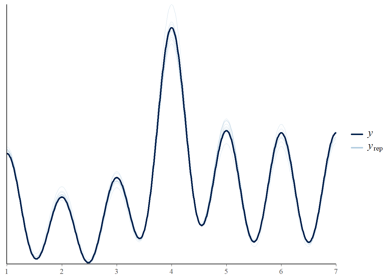
1 (0.0%) p_waic estimates greater than 0.4. We recommend trying loo instead. pp_check(mod_naive)
pp_check(mod_ind)