Homework - Week 03
Q1
The first two problems are based on the same data. The data in
data(foxes)are 116 foxes from 30 different urban groups in England. These fox groups are like street gangs. Group size (groupsize) varies from 2 to 8 individuals. Each group maintains its own (almost exclusive) urban territory. Some territories are larger than others. Theareavariable encodes this information. Some territories also have moreavgfoodthan others. And food influences theweightof each fox. Assume this DAG:
where F is
avgfood, G isgroupsize, A isarea, and W isweight. Use the backdoor criterion and estimate the total causal influence of A on F. What effect would increasing the area of a territory have on the amount of food inside it?
To estimate the total effect of A on F, we just need to model F ~ A because there are no shared causes.
tar_load(fox)
tar_load(h03_q1_prior)

# look at priors we selected
prior_summary(h03_q1_prior)
prior class coef group resp dpar nlpar lb ub source
normal(0, 0.5) b user
normal(0, 0.5) b area_s (vectorized)
normal(0, 0.5) Intercept user
exponential(1) sigma 0 user# prior predictive
epred <- add_epred_draws(fox, h03_q1_prior, ndraws = 100)
ggplot(epred, aes(x = area_s, y = .epred)) +
geom_line(aes(group=.draw), alpha = 0.1) +
labs(y = "Predicted Food (standardized)", x = "Area (standardized)") +
theme_classic()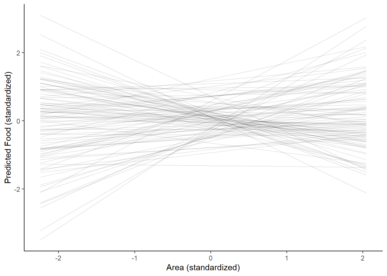
# posterior distribution
tar_load(h03_q1)

# make dataset sequencing from -2 to 2 (reasonable range of values for standardized numbers)
df <- data.frame(area_s = seq(-2, 2, length.out = 1000))

epred_data <- h03_q1 %>%
  epred_draws(df)

# plot slopes
p <- ggplot(data = fox, aes(x = area_s)) +
  stat_lineribbon(aes(x = area_s, y = .epred), data = epred_data) +
  geom_jitter(aes(y = avgfood_s), width = .1, height = 0, alpha = 0.7) +
  scale_fill_brewer(palette = "Greys") +
  theme_classic() +
  scale_y_continuous(limits = c(-2, 2), breaks = c(-2, -1, 0.5, 0, 0.5, 1, 2, 5))

# extract plot breaks on x and y axes
atx <- c(as.numeric(na.omit(layer_scales(p)$x$break_positions())))
aty <- c(as.numeric(na.omit(layer_scales(p)$y$break_positions())))

# unscale axis labels for interpretation
p +
  scale_x_continuous(name = "Area",
                     breaks = atx,
                     labels = round(atx * sd(fox$area) + mean(fox$area), 1))  +
  scale_y_continuous(name = "Average Food",
                     breaks = aty,
                     labels = round(aty * sd(fox$avgfood) + mean(fox$avgfood), 1)) +
  labs(fill = "Credible Interval")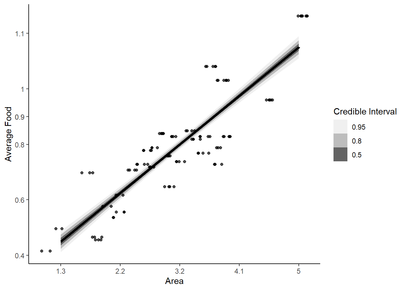
As area of a territory goes up, average food also increases.
Q2
Infer the total causal effect of adding food F to a territory on the weight W of foxes. Can you calculate the causal effect by simulating an intervention on food?
Total effect of food on weight is estimated by modelling W ~ F (no backdoor paths).
tar_load(fox)
tar_load(h03_q2_prior)

# look at priors we selected
prior_summary(h03_q2_prior)
prior class coef group resp dpar nlpar lb ub source
normal(0, 0.5) b user
normal(0, 0.5) b avgfood_s (vectorized)
normal(0, 0.5) Intercept user
exponential(1) sigma 0 user# prior predictive
epred <- add_epred_draws(fox, h03_q2_prior, ndraws = 100)
ggplot(epred, aes(x = avgfood_s, y = .epred)) +
geom_line(aes(group=.draw), alpha = 0.1) +
labs(y = "Predicted Weight (standardized)", x = "Area (standardized)") +
theme_classic()
# posterior distribution
tar_load(h03_q2)

# make dataset sequencing from -2 to 2 (reasonable range of values for standardized numbers)
df <- data.frame(avgfood_s = seq(-2, 2, length.out = 1000))

epred_data <- h03_q2 %>%
  epred_draws(df)

# plot slopes
p <- ggplot(data = fox, aes(x = avgfood_s)) +
  stat_lineribbon(aes(x = avgfood_s, y = .epred), data = epred_data) +
  geom_jitter(aes(y = weight_s), width = .1, height = 0, alpha = 0.7) +
  scale_fill_brewer(palette = "Greys") +
  theme_classic() +
  scale_y_continuous(limits = c(-2, 2), breaks = c(-2, -1, 0.5, 0, 0.5, 1, 2, 5))

# extract plot breaks on x and y axes
atx <- c(as.numeric(na.omit(layer_scales(p)$x$break_positions())))
aty <- c(as.numeric(na.omit(layer_scales(p)$y$break_positions())))

# unscale axis labels for interpretation
p +
  scale_x_continuous(name = "Average Food",
                     breaks = atx,
                     labels = round(atx * sd(fox$avgfood) + mean(fox$avgfood), 1))  +
  scale_y_continuous(name = "Weight",
                     breaks = aty,
                     labels = round(aty * sd(fox$weight) + mean(fox$weight), 1)) +
  labs(fill = "Credible Interval")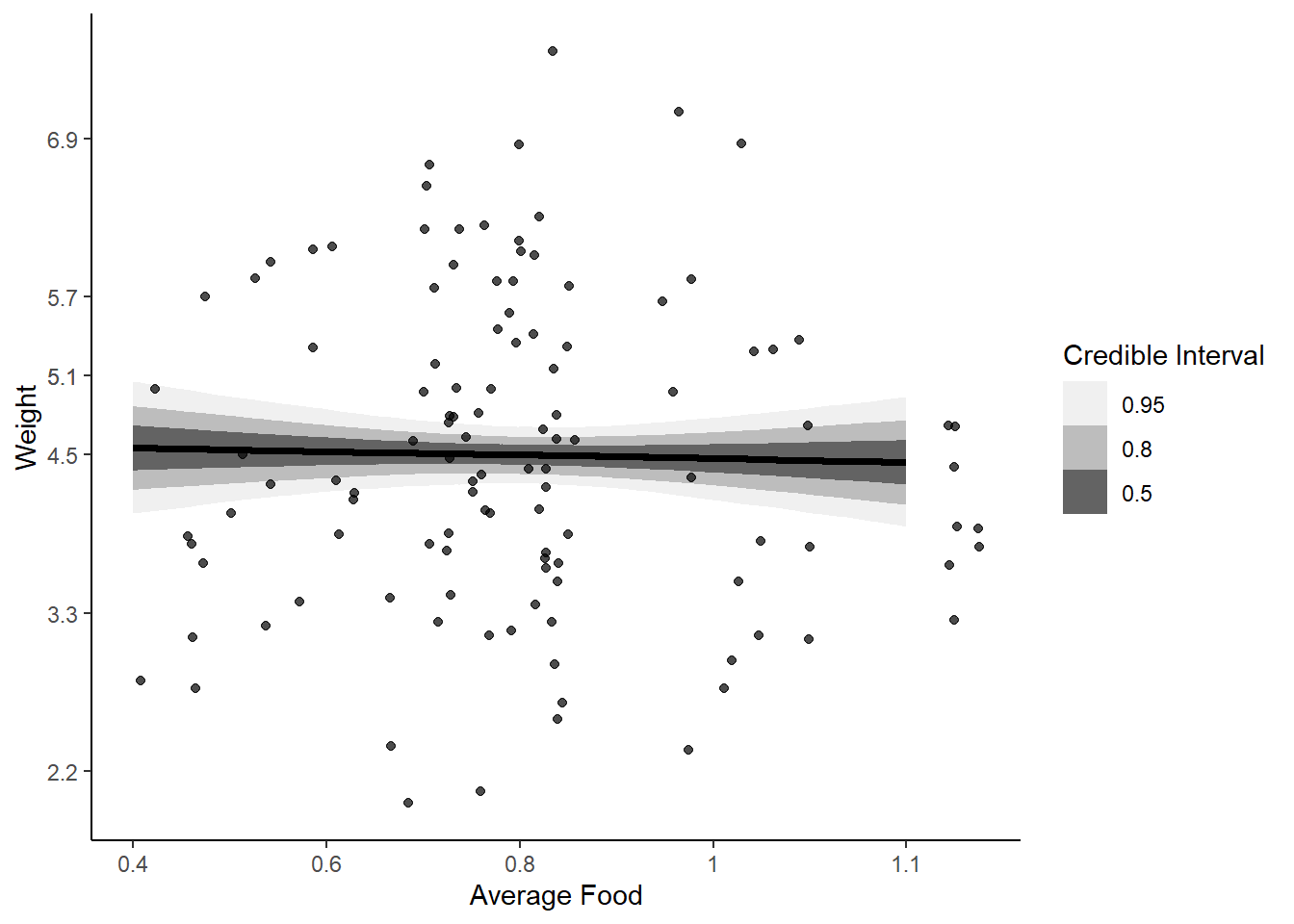
# does slope change at different values of food?
h03_q2 %>%
  emtrends(~ avgfood_s,
           var = "avgfood_s",
           at = list(avgfood_s = c(0, 2)),
           epred = TRUE, re_formula = NA)
avgfood_s avgfood_s.trend lower.HPD upper.HPD
0 -0.0232 -0.205 0.161
2 -0.0232 -0.205 0.161
Point estimate displayed: median
HPD interval probability: 0.95 cont <- h03_q2 %>%
emtrends(~ avgfood_s,
var = "avgfood_s",
at = list(avgfood_s = c(0, 2)),
epred = TRUE, re_formula = NA) %>%
gather_emmeans_draws()
ggplot(cont, aes(x = .value, fill = factor(avgfood_s))) +
stat_halfeye(slab_alpha = 0.75) +
scale_fill_manual(values = c('darkseagreen', 'lightblue')) +
labs(y = "Density", x = "Average marginal effect of a unit increase in avgfood", fill = "avgfood (standardized)") +
theme_classic() +
theme(legend.position = "bottom")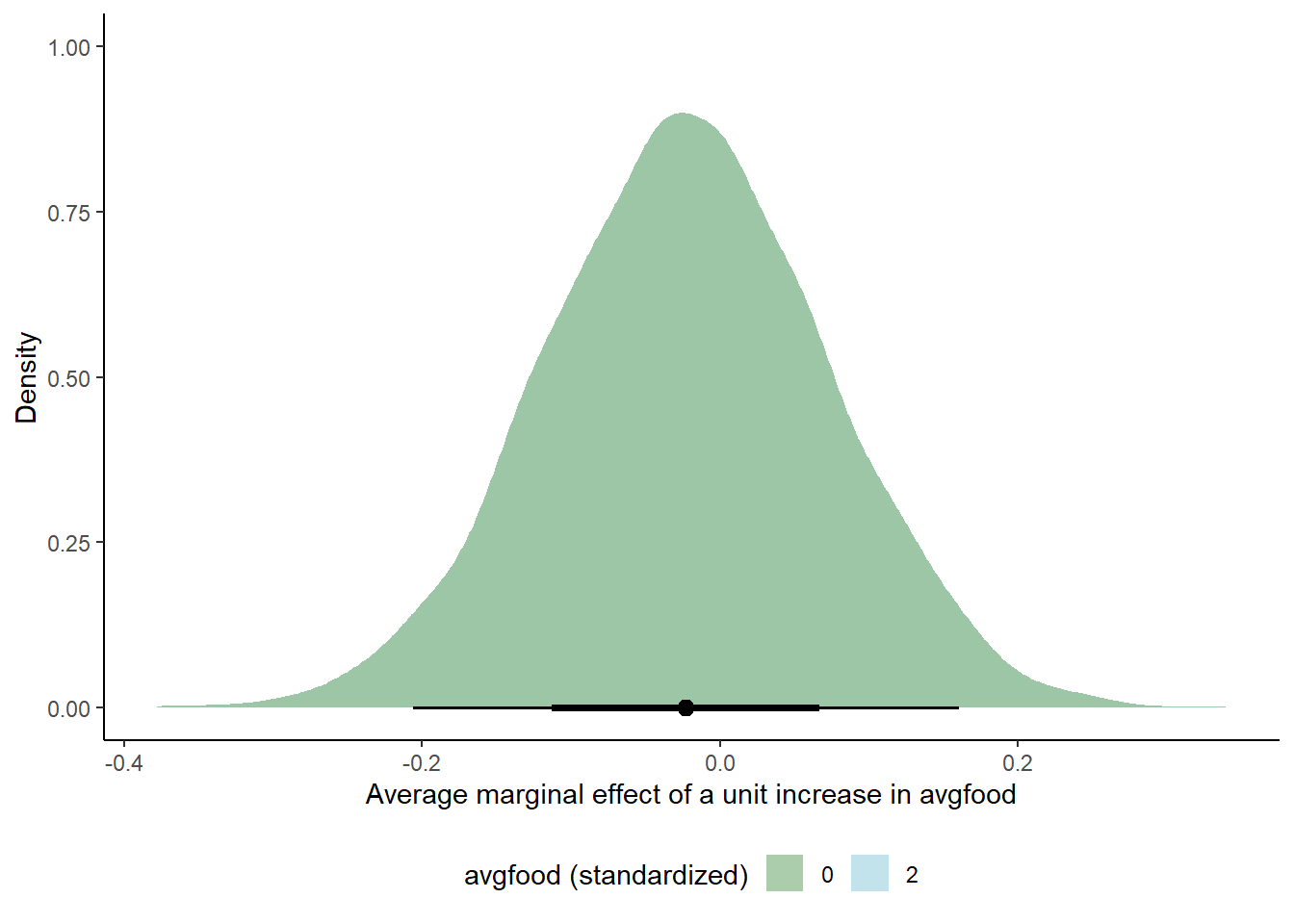
# NO! Linear model, slope doesn't change across different values

# simulate an intervention: calculate the contrast between a lot of food and average amount of food
mf <- data.frame(avgfood_s = 0)
hf <- data.frame(avgfood_s = 1)

med <- h03_q2 %>%
  epred_draws(newdata = mf)

high <- h03_q2 %>%
  epred_draws(newdata = hf)

cont <- data.frame(cont = med$.epred - high$.epred)

ggplot(cont, aes(x = cont)) +
  stat_halfeye() +
  labs(x = "avgfood_s of 0 - avgfood_s of 1", y = "") +
theme_classic() 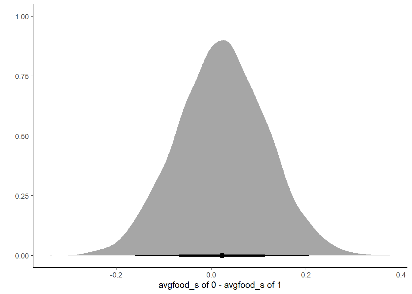
Total effect of food on weight is very small, we see very little effect of increasing food
Q3
Infer the direct causal effect of adding food F to a territory on the weight W of foxes. In light of your estimates from this problem and the previous one, what do you think is going on with these foxes?
Direct causal effect of food on weight requires stratifying by groupsize (G).
tar_load(h03_q3)


# make dataset sequencing from -2 to 2 (reasonable range of values for standardized numbers)
# hold groupsize constant (at average level)
df <- data.frame(avgfood_s = seq(-2, 2, length.out = 1000),
                 groupsize_s = 0)

epred_data <- h03_q3 %>%
  epred_draws(df)

# plot slopes
p <- ggplot(data = fox, aes(x = avgfood_s)) +
  stat_lineribbon(aes(x = avgfood_s, y = .epred), data = epred_data) +
  geom_jitter(aes(y = weight_s), width = .1, height = 0, alpha = 0.7) +
  scale_fill_brewer(palette = "Greys") +
  theme_classic() +
  scale_y_continuous(limits = c(-2, 2), breaks = c(-2, -1, 0.5, 0, 0.5, 1, 2, 5))

# extract plot breaks on x and y axes
atx <- c(as.numeric(na.omit(layer_scales(p)$x$break_positions())))
aty <- c(as.numeric(na.omit(layer_scales(p)$y$break_positions())))

# unscale axis labels for interpretation
p +
  scale_x_continuous(name = "Average Food",
                     breaks = atx,
                     labels = round(atx * sd(fox$avgfood) + mean(fox$avgfood), 1))  +
  scale_y_continuous(name = "Weight",
                     breaks = aty,
                     labels = round(aty * sd(fox$weight) + mean(fox$weight), 1)) +
  labs(fill = "Credible Interval", title = "Group size held constant")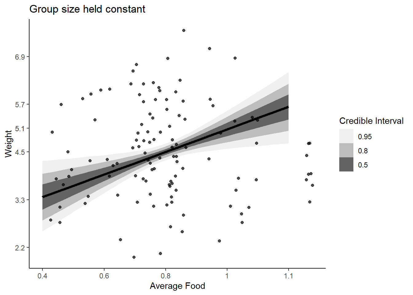
When we stratify by group size, the direct effect of food on weight is strongly positive. Group size may diminish the total effect of food on weight because as avgfood increases, group size increases and the same amount of food is available for each individual, resulting in no change in weight.
Q4 (optional)
Suppose there is an unobserved confound that influences F and G, like this:
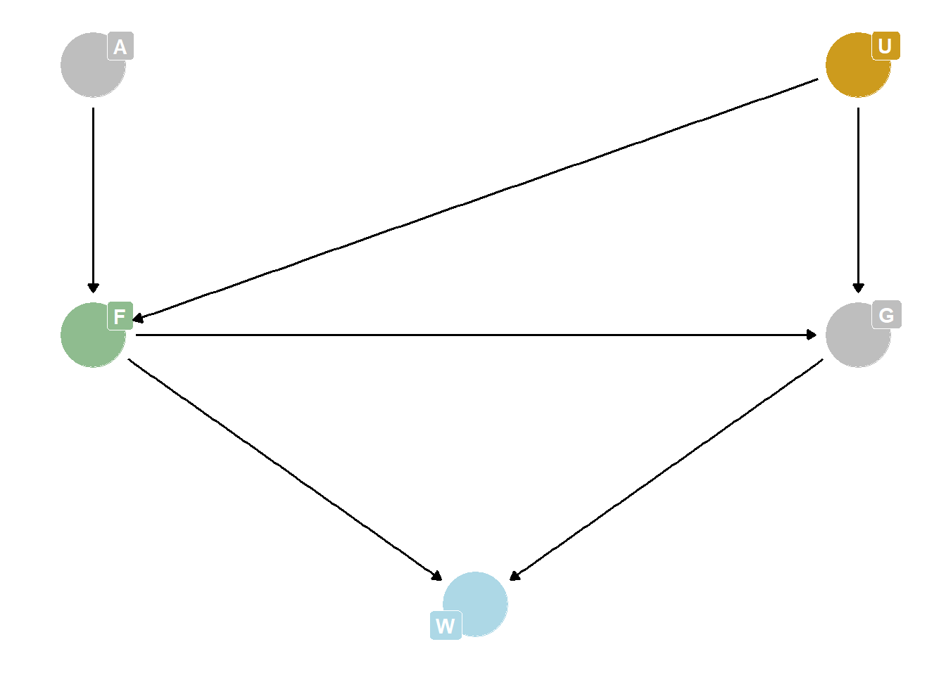
Assuming the DAG above is correct, again estimate both the total and direct causal effects of F on W. What impact does the unobserved confound have?
Total causal effect is impossible to estimate, because you can’t close the backdoor path through U. Direct causal effect is the same, estimated by stratifying on G.