Lecture 08 - Markov chain Monte Carlo

Rose / Thorn

Rose:

Thorn:

Modelling Approaches

• quadratic approximation makes strong assumptions about what the model looks like - approximately Gaussian

• MCMC is intensive but with less assumptions and more flexible

Markov chain Monte Carlo

• chain: sequence of draws from distribution

• Markov chain: history doesn’t matter, just where you are now

• Monte Carlo: random simulation

Hamiltonian Monte Carlo

• probability space is essentially a skate park
• uses random pathways that follow the distribution of the variables

dag <- dagify(
  S ~ Q + J + X,
  Q ~ X,
  J ~ Z,
  outcome = 'S',
  latent = 'Q',
    coords = list(x = c(Q = 0, X = 0, S = 1, J = 1, Z = 2),
                y = c(X = 0, J = 0, Z = 0, Q = 1, S = 1))
)

ggdag(dag) + theme_dag()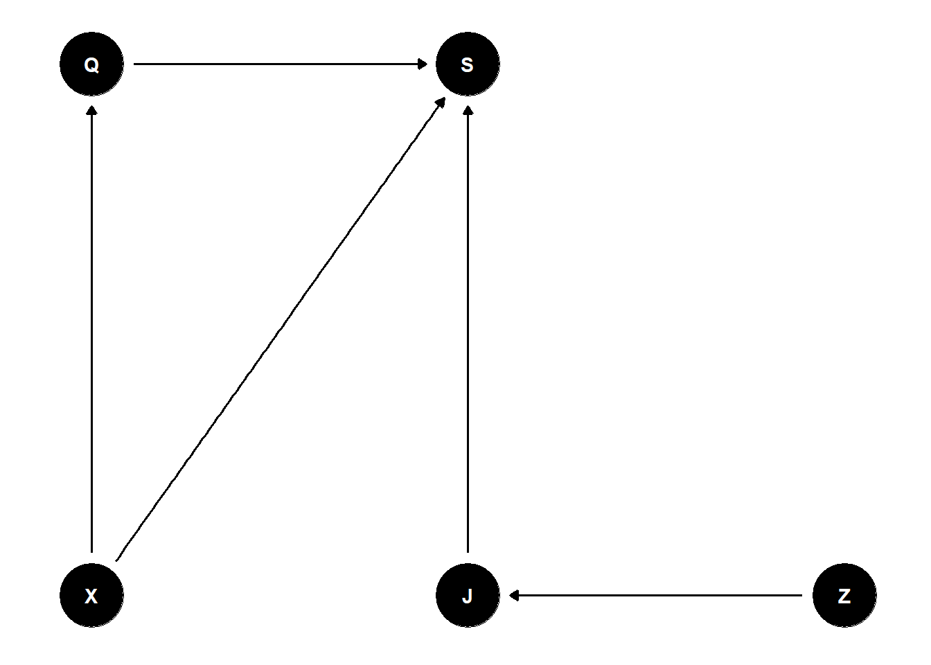

• Estimand: association between wine quality and wine origin. Stratify by judge for efficiency.

data(Wines2012)
d <- Wines2012

dat <- list(
  S = standardize(d$score),
  J = as.numeric(d$judge), 
  W = as.numeric(d$wine),
  X = ifelse(d$wine.amer == 1,1,2),
  Z = ifelse(d$judge.amer == 1,1,2)
)

mQ <- ulam(alist(
  S ~ dnorm(mu, sigma), 
  mu <- Q[W],
  Q[W] ~ dnorm(0, 1), 
  sigma ~ dexp(1)),
  data = dat, chains = 4, cores = 4)

precis(mQ, 2)

• trace plots: visualization of the Markov chain

• want more than one chain in order to check convergence

  • convergence: each chain explores the right distribution and the same distribution

• R-hat is chain convergence diagnostic

  • variance ratio

  • if chains do converge, beginning of the chain and end of chain should be exploring the same place and therefore the chain is stationary

  • as total variance (among chains) approaches average variance within chains, R-hat approaches 1

  • if chains were exploring different regions, the total variance would be bigger and Rhat is larger than 1

  • does not guarantee convergence but gives an idea that the chains are working when ~ 1

• n_eff = effective samples

  • approximation of how long the chain would be if each sample was completely independent of the one before it (perfectly uncorrelated, truly random)

  • when samples are autocorrelated, you have fewer effective samples

  • typically n_eff is smaller than number of samples you actually took

    • because perfect chain will need fewer samples/be shorter

mQO <- ulam(alist(
  S ~ dnorm(mu, sigma), 
  mu <- Q[W] + O[X],
  Q[W] ~ dnorm(0, 1),
  O[X] ~ dnorm(0, 1),
  sigma ~ dexp(1)),
  data = dat, chains = 4, cores = 4)

plot(precis(mQO, 2))

mQOJ <- ulam(alist(
  S ~ dnorm(mu, sigma), 
  mu <- (Q[W] + O[X] - H[J])*D[J],
  Q[W] ~ dnorm(0, 1),
  O[X] ~ dnorm(0, 1),
  H[J] ~ dnorm(0, 1),
  D[J] ~ dexp(1),
  sigma ~ dexp(1)),
  data = dat, chains = 4, cores = 4)

plot(precis(mQOJ, 2))

• adding judges adds information to the model and allows for better estimates

• often if there is an issue, it is with your model

  • loop back to basic scientific questions and assumptions

  • divergent transitions are one of the signs of this - “rejected proposal”